Seg2Dgel Reference Manual
Seg2Dgel Reference Manual
Seg2Dgel is a Java 2D electrophoreic gel segmentation program for
finding and measuring the integrated density and position of spots in
a gel or similar type of data. Figure 1 shows the home page. It is a
one of the modules in the Open2Dprot project.
The program may be run either interactively (-gui) or under an OS
shell command to implement batch (-nogui). If the -gui mode is used,
after the segmentation is finished, the user has the option of
interactively viewing any of the images used by the segmenter and
querying them for quantified spot data or look at small pixel windows
(3x3 to 21x21 pixels) of the image data and the intermediate images
used in the segmentation. The user may also modify the input switch
options and save the new options in a "Seg2Dgel.properties" file in
the current project directory so that it may be used as the default
switch options in subsequent running of the segmenter.
NOTE: the "Seg2Dgel.properties" file is not currently used in the
current version.
The application looks up the sample in the accession database (if the
latter exists in xml/accession.xml or as specified using the
-accessionFile switch). It then gets additional information about the
sample including the computing window and the grayscale calibration if they exist in the
database.
If no accession database entry exists or there is no accession database
(indicated by using the -noAccessionDB or
-default:NO-DATABASE switch on startup), then the entire image
is analyzed and no grayscale calibration is used and spot density
is the sum of the gray values in a spot. The sample name is the
image name without the file path or file extension. The
-default:NO-DATABASE switch also sets other switches to
a specific default, so read the options in the list of switches before
you use it. See the example for some
typical command line switches to use.
The Open2Dprot
http://open2dprot.sourceforge.net/Accession pipeline module is
used for entering samples into the accession database.
[Status: The Open2Dprot Accession module program is available to create
and edit an accession file. Alternatively, the accession database
could be created or edited manually as either XML (accession.xml), or
tab-delimited text (accession.txt) with a text editor or Excel.]
Input images may be in TIFF (.tif, .tiff), JPEG (.jpg), GIF (.gif), or
PPX (.ppx GELLAB-II) format. TIFF images may be 8-bits/pixel through
16-bits/pixel, whereas JPEG, GIF, and PPX are 8-bit images. Gray
values in the images files have black as a 0 pixel value. Gray values
are mapped to 0 for white and maximum pixel value for black. This
allows us to compute integrated density/spot (if the gel is calibrated
in optical density) or integrated grayscale/spot. For purposes of this
documentation, assume that the input image names without the file
extension is gelName so in the case of the example plasma27.tif
file name, gelName would be "plasma27" would be the sample
name.
For color images, the RGB data is first mapped to grayscale using the
NTSC color to grayscale transform (gray = 0.33*red + 0.50*green +
0.17*blue) [FUTURE].
The input gel image file is kept in the
user-project-directory/ppx/ sub-directory. If it is not in that
directory, then it will prompt you for the name of a project directory
and create it and the sub-directories if they do not already exist.
Then it will copy your input file to project directory so that the
database is consistent and may be used by the other Open2Dprot
analysis pipeline programs.
[STATUS: currently NTSC conversion is not available.]
The data output file is called the Sample Spot-list File (SSF) and is
saved in the user-project-directory/xml/ directory. The
generated name the same as the base name of the image file but with a
different extension depending on the output format. The possible
extensions are: .ssf (for ASCII format compatible with GELLAB-II),
.xml (XML format), and .txt (tab-delimited format). The format is
specified by the -ssfFormat:{F | G | T |
X} command line switch.
[STATUS: currently XML -ssfFormat:X is the default format, but
the XML generated will change with new changes in MIAPE.]
The segmented output image is
[STATUS: currently the output images are GIF (.gif) images.]
The grayscale to calibration grayscale map is be specified by pairs of
calibration (grayscale-values, calibrated-units-values). This is then
used to construct a piece-wise linear calibration map to use as a table
lookup to map grayscale values to calibration values. If the mapping is
reasonably well behaved, for a reasonably smooth curve, 15 to 25
points will suffice.
The computing window is the valid region in
image that should be segmented. Regions outside of this are
ignored.
[STATUS: Calibrations can be optionally be specified in the accession
database file if it exists. The calibration procedure, if available, can
be performed in the
http://open2dprot.sourceforge.net/Accession pipeline module of
Open2Dprot. Accession allows users to generate and add the calibration
to the accession database for samples.]
The -averageOD switch does the image averaging computations in OD
space rather than grayscale space.
The averaging filters are defined as follows:
The -differenceOD switch does the image Laplacian computations in OD
space rather than grayscale space.
The Laplacian filters are defined as follows where Where, a CC pixel
is defined as an UNLABELED_CC_CODE (i.e., 1) if both dX and dY < 0,
else it is define as a background pixe BKGRD_CODE (i.e., 0). The
magnitude is computed as either the city-block distance(faster) or
Euclidean distance of (dX, dY).
Use of Line Laplacian for detecting "spots" in 2D LC-MS images
There is an experimental line laplacian that we are optimizing for use
with 2D LC-MS images. It is specified as
-laplace:H,height,width for horizontal lines and as
-laplace:V,height,width for vertical lines. The values
for height and width are image dependent and are currently being
titrated on a variety of images. You use either the horizontal or the
vertical filter - not both. The screen shots in Figures 3 shows the
use of a horizontal filter on low resolution 2D-LC-MS data (thanks to
Laboratory of Proteomics and Analytical Technologies,
NCI-Frederick).
[STATUS: Not currently available - being debugged.]
There are situations where some spots are merged into single spots.
Examples include post-modification charge trains of high concentration
spots. Visual inspection of the segmented gels makes it easy to split
these spots by matching opposing concavities.
The -splitSpots:{B | R | T},minCCsplitSize
switch will try to split large spots based on an 'B'oundary analysis
or 'R'egion analysis or a 'T'hreshold analysis based on Miller and
Olson's spot splitting algorithm [A. Olson, M. Miller, 1989]. This is
useful in some cases where spots are not resolved which should have
been. A useful starting value for minCCsplitSize should be at least 15
pixels. Note that the other minimim spot sizing parameter - the
primary minimum spot sizing parameter set by
-ccMinSize:nbrPixels, with default size 2 pixels, ignores spots
or subspots less than nbrPixels. Normally the -splitSpots switch is
not used.
The algorithm first performs two checks to see if a spot is a candidate
for splitting:
[STATUS: note we currently generate .gif images rather than .jpg, but
this will change.]
For an image with nCols X nRows, the default computing window is set
to [2:nCols-2 x 2:nRows-2] if it is not defined. You can set the
computing window using the -cw:x1,x2,y1,y2 command line switch. In
any case it is clipped to [2:pixWidth-2 x 2:pixHeight-2] where the
image is of size pixWidth x pixHeight.
If you specify an image to be semented, it will check whether it is in
a ppx/ subdirectory. If not, it will ask you if you want to create a
project directory and will then set up the following four directories
and copy your image into the ppx/ directory. You can also use the
-projDir:user-project-directory switch to specify a (possibly
new) project directory.
If you are using the Windows Seg2Dgel.exe file or clicking on the
Seg2Dgel.jar file, you can't change the default startup memory.
If you are using the Seg2Dgel.jar in a script using the java interpreter
as in the following example which uses the -Xmx256M
(specifying using 256Mbytes at startup). Change 256 to a larger size
if you want to increase startup memory.
All logged output is sent to the report window in a scrollable text
window that may be saved or used for cut and paste operations. A set
of command buttons at the bottom of the window are replicates of
commands in the menus, but are easier to access. They include the
following functions:
The "-histGUI" ("-nohistGUI) switch can be used to add (remove) it
from the command line. The (View | Add histogram to Image
Viewer) checkbox menu command or the popup options wizard window
can also be used to change it.
You can do rudimentary spot data filtering (if enabled in the
Histogram menu of the Image Viewer) where spots passing the filter are
indicated in the image. You can click on a bin in the histogram and
the filter will show spots (with a cyan "+") GEQ or LEQ the bin value
you selected. Clicking on the histogram, will select that bin and
display the corresponding data for that bin. Note, if you enable the
The documentation is kept on the Internet at
http://open2dprot.sourceforge.net/Seg2Dgel. Normally, these help
commands should pop up a Web browser that directly points to the Web
page on the http://open2dprot.sourceforge.net/Seg2Dgel site. If your
browser is not configured correctly, it may not be able to be launched
directly from the Seg2Dgel program. Instead, just go to the Web site
with your Web browser and look up the information there.
An Internet connection is required to download the program from the
Open2Dprot Seg2Dgel Web site. New versions of the program and
associated demo data will become available on this Web site and can be
uploaded to your computer using the various
(File | Update from Web server | ...) menu commands. If you
have obtained the installer software that someone else downloaded and
gave to you, then you do not need the Internet connection to install
the program. We currently distribute Seg2Dgel so that it uses up to
256Mb. See discussion on increasing memory.
Any case-independent switch may be negated by preceeding it with
a 'no' eg. '-noinfo'.
The command line syntax used to invoke it is:
The following examples using switches might be useful:
You can these images in the list below or view all of the screen shots in a
single Web page.
Command line scripts to run the GUI version on one sample are in the
second example and
forth example. These may be downloaded
from
demo-Seg2DgelGUI.bat and
demo-Seg2DgelGUI.sh.
The data for these scripts is in the demo/ directory available with the
installation which also includes the scripts.
Alternatively, you can download the demo data from the Files Mirror as
Demo.Z.
The installation packages are available from the
Files mirror
under the Seg2Dgel releases.

Figure 1. Home page for the Seg2Dgel program.
The Web site, at
http://open2dprot.sourceforge.net/Seg2Dgel contains the software
(with downloadable binaries and source code), as well as
documentation.

Figure 2. Screen view of the Seg2Dgel program Graphical User Interface.
This screen shot shows the status after a segmentation
of the demo gel (Human-AML 512x512 8-bit pixels) has completed. The
sizing parameters are shown at the top. Next the summary statistics is
reported. This is followed by a list of generated files (spot list and
segmented spot images). Finally, since the timer was enabled, it gives
a breakdown of how much time was spent in different parts of the
program. [This was run on a 1Ghz pentium-4 Windows 2000 system.] The
pull-down menus at the top of the window used
to invoke File operations, Edit, View, Quantify (i.e. spot
segmentation), and Help commands. Although, the button commandss at
the bottom of the window are also available in the menus, they are
replicated as buttons for convenience. The Clear button will
clear the window. SaveAs will let you save the text in a text
file. The Edit options button pops up a window to let you edit
the options including the gel name, computing window, sizing
thresholds etc. The Segment button starts the segmenter on the
current options. You can stop the segmenter by pressing the Stop
program button. After you have segmented the image, you can review
the images by pressing the Image Viewer to popup the image
viewing window. A status area appears in the lower left corner and
reports the current state of the segmenter during an analysis. It
shows "Done" since the segmentation had completed.
1. Introduction
Seg2Dgel is a Java 2D electrophoresis gel segmentation program for
finding and measuring the integrated density and position of spots in
a sample gel. We are adding other features to enable it to segment 2D
LC-MS data presented as images. Seg2Dgel is part of the Open2Dprot
project (
http://open2dprot.sourceforge.net/). The segmentation is
performed on a computing window region of interest (ROI) of a 2D gel
image file. It uses the second derivative (laplacian) magnitude and
direction of the gaussian-smoothed gel image as well as neighborhood
connectivity properties in determining spot extents.Project directory structure for Open2Dprot and Seg2Dgel
All Open2Dprot programs assume a project directory structure. This
must exist for the program to proceed. You can either create the
structure prior to running any of the programs or you can create it on
the fly using the -projDir:user-project-directory. It will lookup
and/or create the following sub-directories:
 user-project-directory/batch/ - batch temporary files - [not used]
 user-project-directory/cache/ - cache files - [not used]
 user-project-directory/ppx/ - original input image files
 user-project-directory/rdbmx/ - RDBMS CSD database files - [not used]
 user-project-directory/tmp/ - generated derived image files
 user-project-directory/xml/ - accession DB, generate SSF files
The use of these directories is discussed in the rest of this
document.Input gel image file
The sample to be segmented is specified by its image file name using
the -sample switch with or without the file extension (e.g.,
-sample:plasma27.tif or -sample:plasma27). The file extension is
determined by looking up the image in the ppx/ project subdirectory at
run time. Output spot list file in Sample Spot-list File (SSF)
The output is a quantified spot list in various ASCII formats
including XML and tab-delimited as well as the historical GELLAB-II
SSF formats. Images may be generated (a the user's option) to view
the segmented spots and various intermediate images used by
Seg2Dgel.Output images files
You may save various images used in segmenting the input image. These
are mapped to 8-bits reguardless of the actual internal resolution and
saved as 8-bit JPEG (.jpg) in the user-project-directory/tmp/
directory at the same directory level as the input image file.Spot overlays in the output image
Spots may be indicated in the 'seg' or 'restOf' output images in
several ways. The -drawDot:{O | Z} switch will draw a
dot, the -drawDot:{O | Z} switch will draw a plus ("+"),
and the -drawBoundary:{O | Z} switch will draw a
boundary. It will draw it in the default 'Z' (segmented) image rather
than in a copy of the 'O'riginal image. The
-drawMinEnclRect:{P|O} switch to draw minimum enclosing
rectangle spot overlays.
Calibration grayscale data in the accession database file
If the grayscale is to be calibrated in particular units, this is done
through the entry for the sample in the accession database. The accession
database entry specifies 4 items: a short list (15 to 25 entries) of
calibration values sorted in assending order, a corresponding list of
gray values also in assending order, calibration units (e.g., "optical
density"), and an abbreviation for the units (e.g., "od"). It is
assumed that the image pixels when mapped to calibration units (such
as Optical Density (OD), Counts-Per-Minute (CPM), etc.) will be
stochiometric so that a spot's integrated density corresponds to the
spot's protein concentration. How well this relationship holds helps
determine the accuracy of the quantification. We use a piecewise-linear
extrapolation to map this list into a gray-scale to calibration-units
lookup table. This is used in all image pixel density computations so
that the computations are performed in calibration-units space rather
than grayscale space for more accurate quantification. The Open2Dprot
http://open2dprot.sourceforge.net/Accession pipeline module is
used for editing and defining this calibration data for each sample.Use of calibration data during analysis
If there is a grayscale to optical density (or other units,
counts/minute, etc.) calibration, it is assumed that it is specified
in the accession database. The accession database may be read if it
exists when the sample is processed. A calibration entry consists of
calibration information including grayscale to optical density,
microns/pixel, the computing window where the sample image is to be
segmented, etc. The calibration maps gray scale pixel values to a
calibrated value (such as optical density, counts/minute, etc.) that
may correspond to protein concentration if the protein sample
quantification method (dye, radioautography, etc.) and the scanner
have a reasonably linear or know mapping. If there is no calibration
specified, it does a 1:1 mapping of grayscale to "Grayscale" units.2. Seg2Dgel spot segmentation algorithm
The segmentation algorithm is described in two parts. The first part
describes the global image processing operations. The send part
describes individual spot segmentation operations.
The following algorithm describes the processing each spot undergoes
during its segmentation.
The steps in finding the final PCC for the current spot are enumerated
as follows. This algorithm is iterated for each spot as it traverses
down the image in a raster pattern.
It uses the final PCC to compute spot features including:
    density weighted centroid: (xMom, yMom),
    standard deviation and covariance spot size: (Sx, Sy, Sxy)
    integrated density: density
    integrated density: meanDensity
    spot area: area
    max and min OD: (minD, maxD)
    M.E.R. (minimum enclosing rectangle): [merX1:merX2, merY1:merY2]
Using these features, it estimates and includes the spot volume
computed as
volume = 4 * Sqrt(PI) * maxD * Sx * Sy.
It then filters out spots that do not pass the threshold ranges test
(area in [a1:a2]) and (density in [d1:d2]) and (od diff in [o1:o2])
The od diff is (maxD - minD). The thresholds may be set by the command
line switches
-thrArea:a1,a2 -thrDensity:d1,d2 -thrRange:o1,o2
After all spots are found, it computes a background image from the
original image less the spots. This is then used to compute a zonal notch
filter background image from this image. It uses the background image as
a table lookup of backgrounds at the centroids of the spots. It also adds
background related spot features including:
    mean background density: meanBkgrd
    background density: densityBkgrd
It then computes the density corrected for background,
density' = density - densityBkgrd * area
for each spot and then retests Density' agains the lower density limit
t1 -thrDensity:t1,t2. Spots failing this test are then
removed. It then adds the spot feature:
density'
Image smoothing operations
The first image convolution operation performed is needed to smooth
the image. If the image is not sufficiently smoothed, it will not find
the edges of the spots correctly. segmentation: Gaussian lowpass
filter smoothing and a Laplacian. The Gaussian smoothing size is
specified by one of the following switches -lowpassFilter:{3 |
5 | 7 | 13} size (i.e., 3x3, 5x5, 7x7, 13x13).
If you do not specify the filter, then it is defaulted from the image
size.
  a) use -lowpassFilter:3 switch
      1 2 1
      2 4 2  divided by 16
      1 2 1

  b) for the -lowpassFilter:5 switch
      1 1 2 1 1
      1 2 4 2 1
      2 4 8 4 2   divided by 52
      1 2 4 2 1
      1 1 2 1 1

  c) for the -lowpassFilter:7 filter (Miller & Olson)
      4  -6  -12  -14  -12   -6  4
     -6   9   18   21   18    9 -6
     -12 18   36   42   36   18 -12
     -14 21   42   49   42   21 -14  /441
     -12 18   36   42   36   18 -12
     -6   9   18   21   18    9 -6
      4  -6  -12  -14  -12   -6  4

   d) -lowpassFilter:13,size.
      Gaussian filter Cij is convolved with image data Jij and
      then normalized
     j11 ... j1h      c11 ... c1h
         ...      *       ...
     jd1 ... jdh      cd1 ... cdh
Image Laplacian operations
Similarly, there are three symmetric Laplacian edge detection filters:
3x3, 5x5 and BusseFilter specified by -laplacian:3,
-laplacian:5, and -laplacian:B,gridSize,mode
where mode is P or C. In the Busse Laplacian, the
gridSize defaults to 3x3. If the mode being 'P', pixel weights are
used, for 'C' 3x3 averaged pixel weights are used. The default
Laplacian is -laplacian:3 is the default 3x3 laplacian. For a
250 microns/pixel image, the -lowpassFilter:7 filter is optimal while
the -laplacian:13 one is better for a 170 microns/pixel image.
In addition, there are two
line-filter Laplacian filters useful for detecting short line-like
objects (as in some 2D LC-MS images).
  a) use -laplacian:3 switch
         0  0  0
    dX = 1 -2  1
         0  0  0

         0  1  0
    dY = 0 -2  0
         0  1  0

  b) use -laplacian:5 switch
         0  0  0  0  0
    dX = 1  1 -4  1  1
         0  0  0  0  0

         0  1  0
         0  1  0
    dY = 0 -4  0
         0  1  0
         0  1  0

  c) use -laplacian:B,mode,gridSize switch.
   This switch is like -laplace:3 but with a pixel spacing specified
   by gridSize and the mode determines if it a single pixel (P)
   or a 3x3 neighborhood average (C) at that grid spacing. This
   filter is useful for fuzzy or noisy images.
  a) use -laplacian:V,height,width
    The vertical line detector filter using horizonal
    difference with widths (3,5,7,9) pixels
    =================================================

          0  0  0
    dX3 = 1 -2  1
          1 -2  1
            ...
          0  0  0

          0  0  0  0  0
    dX5 = 1  2 -6  2  1
          1  2 -6  2  1
              ...
          0  0  0  0  0

          0  0  0  0  0  0  0
    dX7 = 1  2  3 -12 3  2  1
          1  2  3 -12 3  2  1
                  ...
          0  0  0  0  0  0  0

          0  0  0  0  0  0  0  0  0
    dX9 = 1  2  3  4 -20 4  3  2  1
          1  2  3  4 -20 4  3  2  1
                   ...
          0  0  0  0  0  0  0  0  0

  b) use -laplacian:H,height,width
    The horizontal line detector filter using vertical
    difference with heights (3,5,7,9) pixels
    ==================================================

          0  1  1 ... 0
    dY3 = 0 -2 -2 ... 0
          0  1  1 ... 0

          0  1  1 ... 0
          0  2  2 ... 0
    dY5 = 0 -6 -6 ... 0
          0  2  2 ... 0
          0  1  1 ... 0

          0  1   1  ... 0
          0  2   2  ... 0
          0  3   3  ... 0
    dY7 = 0 -12 -12 ... 0
          0  3   3  ... 0
          0  2   2  ... 0
          0  1   1  ... 0

          0  1   1  ... 0
          0  2   2  ... 0
          0  3   3  ... 0
          0  4   4  ... 0
    dY9 = 0 -20 -20 ... 0
          0  4   4  ... 0
          0  3   3  ... 0
          0  2   2  ... 0
          0  1   1  ... 0
Handling saturated spots
The -saturateSpots:percentThreshold option will try to find
saturated spots greater than percent threshold of the darkest pixel
(default 0.95). Note that integrated density values for these spots
will not be accurate. Normally the -saturateSpots switch is not
used.Handling the splitting of spots segmented as one spot
 (1) check if FBL CC spot meets minimum CC size criteria and
 (2) check whether split it using one of the following alternative
     heuristics:
    BOUNDARY ANALYSIS:
          look for notch pairs and break apart the spot
          by drawing white between the well-formed notch pair points
          and then find the FBL again!
    THRESHOLDING:
         if splitting a spot and the sub-spot i to be used has
         CCarea[i] < Tb, then merge all adjacent subspots j that also
         have CCarea[j] < Tb.
[STATUS: Not currently available - being debugged.]Image usage within Seg2Dgel
The seven images are called pix1 through pix7 that are allocated as
follows as buffer pointers. Images are generally create when needed
and deleted when finished to save memory. However, if you are using
the -gui option, the images are not removed so you can access them
more easily with the Image Viewer. The pix5 image is not generated
unless the -segmentedPixOutFile is specified. The pix7 image is not
generated unless the -restOfPixOutFile is specified. The pix2, pix3,
pix4 images are saved if the -ctlCorePixOutputFile switch is specified.
All of the pix images are 16-bits except pix3 which is 32-bits (for now)
because of 32-bit CC coding to be used in the future.
  pix1 is original image                          ppx/gelName.pixFileExtn>
  pix2 is magnitude 2nd derivative image          tmp/gelName-mag.jpg
  pix3 is directional derivative central core     tmp/gelName-cc.jpg
  pix4 is average of the original image           tmp/gelName-avg.jpg
  pix5 is segmented output image                  tmp/gelName-seg.jpg
  pix6 is background OD notch filter image        tmp/gelName-bkg.jpg
  pix7 is rest-of image = original - segmented    tmp/gelName-rest.jpg
Propagated Central core image coding scheme for 8-bit images
The following is the current propagated central core (PCC) coding scheme.
NOTE: This will change when we go to a more robust 16-bit encoding.
 BKGRD_CODE           0           - background pixel
 UNLABELED_CC_CODE    1           - unlabeled central core pixel
 MIN_CC_CODE          2           - minimum labeled central core pixel
 MAX_CC_CODE          99          - maximum labeled central core pixel
 PCC_BASE_CODE        100         - guard region splitting previously
                                    merged spots
 MIN_PCC_CODE         102         - min. labeled prop. central core pixel
 MAX_PCC_CODE         199         - max. labeled prop. central core pixel
 KILL_SPOT_CODE       254         - deleted spot in central core
                                    if NEQ sizing (0 if -noDelete).
 ISOLATED_PIXEL_CODE  255         - isolated pixel or non
                                    4-ngh connected pixel
3. Running Seg2Dgel and specifying parameter options via the
command line
The program may be run either interactively (-gui) with a graphical
user interface (GUI) or under an OS shell command to implement batch
(-nogui) depending on how it was started. In the former case, after
the segmentation is finished, the user has the option of interactively
viewing any of the images used by the segmenter and querying them for
quantified spot data or look at small pixel windows (3x3 to 21x21
pixels) of the image data. The user may also modify the input switch
options and save the new options in a "Seg2Dgel.properties" file in the
current project directory so that it may be used as the default switch
options in subsequent running of the segmenter.
All options including the input image to be segmented are specified
via GNU/Unix style switches on the command line (-switch{optional
:parameters} and its negation as -noswitch). However, if
GUI mode is used, you can interactively specify the switches and their
options.
The computing window ROI size
The computing window is a rectangular region in the image that is
considered valid and that spots in this region should be segmented.
Any region outside of this window is ignored.Local Folders and files created and used by Seg2Dgel
When Seg2Dgel is first started, it will check for the following folders
and files in the installation directory and create them if they can
not be found.
Special debugging options -debug and -pixdump switches
Two special switches are available for debugging Seg2Dgel and
for investigating failure modes of particular spots to not
segment correctly for some gels. This is meant only for those
willing to delve into the source code.
Sg2Dgel command-line arguments switch usage
The command line arguements usage is:
Seg2Dgel input-image-file [< optional switches >]
The complete list of switches is given
later in this manual and as well as some examples of typical sets of switches. The
user defined default switches may be specified as a resource string
'Seg2Dgel.properties' file saved in the project directory. For
example:
       -lowpassFilter:3 -laplace:B,C,3 -saturatedPropSpot:99.7 \
       -bkgrdSize:64 -bkgrdCorrection -restOfPixOutputFile \
       -ccMinSize:4 -drawPlus:O
Options wizard window for setting the command line switches
If you invoke the Edit options button in the Report window (or
from the Edit menu), it will popup an options wizard shown in Figure 3.
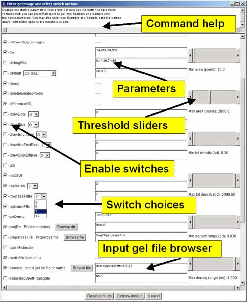
Figure 3. Screen view of the popup options wizard window for
setting the command line switches, parameter and specifying a gel
input image file.
All of the command-line input switches (symbols
starting with a '-') are available in the scrollable window. Switches
are checked if they are enabled and if the switch requires a value,
the current value is shown in the data entry window to its right. On
the right are several threshold sliders for the upper (max) and lower
(min) sizing ranges for several parameters including area, density,
and OD range which set the values for switches
-ccMinSize:minNbrPixels,
-saturatedSpot:percentSaturation, -thrArea:a1,a2,
-thrDensity:d1,d2 and -thrRange:o1,o2. At the top is a
Browse file button to use for specifying a different gel input
image file. There is a Browse dir button to use for specifying
a different project directory. Clicking on any option switchs will
show a short help message associated with that switch at the top of
the window. Pressing the Set new default button will pass the
new options values back to Seg2Dgel. To use the new values, press the
Segment button in the main Report Window to resegment the gel
using the new values.
Updating Seg2Dgel from the Open2Dprot Web server using -update switch
As new versions of Seg2Dgel are developed and put on the Web server,
a more efficient way of updating your version is to use the -update
commands. There are four options:
        -update:program      to update the program jar file
        -update:demo         to update the demonstration files
        -update:doc          to update the documentation files

        -update:all          to update all of the above
After updating the program, it should be exited and restarted for the
new program to take effect. Increasing or decreasing the allowable memory used by Seg2Dgel
If you are working with very large images that require a lot of memory,
you might want to increase the memory available at startup.
java -Xmx256M -jar Seg2Dgel.jar {additional command line args}
4. Command and Report Window - the command center
Seg2Dgel is designed to be used efficiently in a batch mode with
minimal command line output. It is also designed to optionally provide
a graphical user interface (GUI) which creates a Report Window that captures a report
of the segmenter output as well as additional output directed to it by
the user. There are a set of pull-down menus
as well as a set of buttons for often used functions.
5. Pull-down menus in the Graphical User Interface (GUI)
The menu bar a the top of the Report Window contains five menus.
Menu notation
In the following menus, selections that are sub-menus are
indicated by a '![]() '. Selections prefaced with a '
'. Selections prefaced with a '![]() ' and indicate '
' and indicate '![]() ' indicate that the command is a checkbox
that is enabled and disabled respectively. Selections prefaced with a
'
' indicate that the command is a checkbox
that is enabled and disabled respectively. Selections prefaced with a
'![]() ' and indicate '
' and indicate '![]() ' indicate that the command is a
multiple choice "radio button" that is enabled and disabled
respectively, and that only one member of the group is allowed to be
on at a time. The default values set for an initial database are shown
in the menus. Selections that are not currently available will be
grayed out in the menus of the running program. The command short-cut
notation C-key means to hold the Control key and then
press the specified key.
' indicate that the command is a
multiple choice "radio button" that is enabled and disabled
respectively, and that only one member of the group is allowed to be
on at a time. The default values set for an initial database are shown
in the menus. Selections that are not currently available will be
grayed out in the menus of the running program. The command short-cut
notation C-key means to hold the Control key and then
press the specified key.
5.1 File menu
These commands are used to open the gel to be segmented and other file
operations. The current menus and the menu commands (non-working
commands have a '*' prefix) are listed below. You can use either the
"Edit options" button to popup the Options Window editor to change the
gel input file or the (File menu | Open gel image file)
command.
------------------------------------
------------------------------------
![]() - update Seg2Dgel
programs and data from open2dprot.sourceforge.net/Seg2Dgel
server
- update Seg2Dgel
programs and data from open2dprot.sourceforge.net/Seg2Dgel
server
------------------------------------
5.2 Edit menu
These commands are used to change various defaults. These are saved
when you save the state and when you exit the program.
![]() - change the command
line options
- change the command
line options
------------------------------------
5.3 View menu
This menu contains commands to invoke the Image Viewer popup window
used to inspect the images after segmentation. You have the ability
to modify the Region of Interest (ROI) by redefining it for the (-cw,
-pixdump, and -debug regions). Note: in the Image Viewer first select
the ROI as either CW, -dbug ROI, or -pixdump ROI. Then click on the
upper left-hand corner of the new region and type Control-U. Then
click on the upper lower left-hand corner of the new region and type
Control-L. This will then redefine the selected ROI and use it the
next time you run the segmenter from the Report Window. Figure 4. shows an example of the Image Viewer. See
the Examples - samples of screen
shots in the Demos for more examples and description of the some
of the operations available in the Image Viewer.
![]() Add histogram to Image
Viewer - add a dynamic histogram subwindow to the Image viewer
when it is popped up.
Add histogram to Image
Viewer - add a dynamic histogram subwindow to the Image viewer
when it is popped up.
5.3.1 Histogram display in the Image Viewer window
The Image Viewer, in addition the the image display, also has an
optional dynamic histogram display. This may be useful for setting the
threshold parameters. The user may select a feature from a list
including image density under the region of interest (ROI) as well as
spot features (area, mean background density/spot, mean spot
density/spot, total spot density, total spot D', minD/spot, maxD/spot,
spot density range (maxD - minD)). Horizontal and/or vertical image
line cross-section histograms (i.e. image slices) are also available
via the (View | Horizontal slice) and (View | Vertical
slice) menu commands. ![]() Use drag) checkbox, you can
change the bin by draging the mouse. See the Examples - samples of screen shots in
the Demos for more examples and descriptions for using the
histograms. There is also an example of using the horizontal image
density slice.
Use drag) checkbox, you can
change the bin by draging the mouse. See the Examples - samples of screen shots in
the Demos for more examples and descriptions for using the
histograms. There is also an example of using the horizontal image
density slice.

Figure 4. Example of the Image Viewer popup window. It also shows the histogram of the spot area distribution for
spots inside of the computing window. The histogram may display
various spot features. This shows the spot areas under the computing
window (CW ROI). You may change the ROI after the segmentation using
the (Region-Of-Interest | Set ROI type | CW ROI) menu command
in the Image Viewer. The "Spot area" was selected using the
(Histogram | Histogram data | Spot area) menu command. You may
data filter spots that are have an area greater or equal (GEQ) than
the histogram bin selected by clicking on it are shown in the image on
the left as cyan colored "+" marks. The data filter is enabled by the
(Histogram | ![]() Filter spots by
histogram bin) menu command. You set the The data filter test to
GEQ (or LEQ) the bin by the (Histogram |
Filter spots by
histogram bin) menu command. You set the The data filter test to
GEQ (or LEQ) the bin by the (Histogram | ![]() Test spot data GEQ histogram bin) menu
command. Clicking on the histogram will select that bin and display
the corresponding data for that bin. Note, if you enable the
Test spot data GEQ histogram bin) menu
command. Clicking on the histogram will select that bin and display
the corresponding data for that bin. Note, if you enable the ![]() Use drag) checkbox, you can change
the bin by draging the mouse.
Use drag) checkbox, you can change
the bin by draging the mouse.
5.4 Quantify menu
This menu is used to run the segmenter to perform the analysis.
5.5 Help menu
These commands are used to invoke popup Web browser documentation on
Seg2Dgel. Some of the commands will load local documentation in the
the GUI report window.
![]() - this
reference manual
- this
reference manual
--------------------------------------
--------------------------------------
6. Downloading, installing and running Seg2Dgel
The installation packages are available for
download from the SourceForge Files mirror. Look for the most
recent release named "Seg2Dgel-dist-V.XX.XX.zip". These releases include
the program (both as Windows .exe file and a .jar file), required jar
libraries, demo data, Windows batch and Unix
shell scripts. Download the zip file and put the contents where you want
to install the program. Note that there is a Seg2Dgel.exe
(for Windows program). You might make a short-cut to this to use in more easily
starting the program. Alternatively, you can use the sample .bat and .sh scripts
to run the program explicitly via the java interpreter. Note that this method
assumes that you have Java installed on your computer and that it is at
least JDK (Java Development Kit) or JRE (Java Runtime Environment)
version 1.5.0. If you don't have this, you can download the latest version free
from the java.sun.com Website.
6.3 Running Seg2Dgel
There are several ways to run the program. On Windows, you can start
Seg2Dgel by clicking on the startup icon shown in Figure 5 below.
For Unix systems including MacOS-X, you can start Seg2Dgel from
the command line by running the Seg2Dgel.jar file. If your computer is setup
to execute jar files, just type the jar file. In both systems, you can specify
additional command line arguments in Windows .bat and unix .sh scripts (see
examples below.

Figure 5. Startup icon for Seg2Dgel.
Clicking on the icon starts Seg2Dgel. To start Seg2Dgel, click on the startup
icon shown in Figure 6 below - or you can run the demo-Seg2Dgel.bat
script. For Unix systems including MacOS-X, you can start Seg2Dgel from the
command line by clicking on the Seg2Dgel.jar file or using the
demo-Seg2Dgel.sh script. These two scripts run the program in batch.
There are also GUI versions of the two scripts demo-Seg2Dgel-GUI.bat
and demo-Seg2Dgel-GUI.bat that will pop up a user interface.
You could make short-cuts (Windows) or symbolic-links in Unix to make it
easier to start.
6.4 Requirements: minimum hardware and software requirements
A Windows PC, MacIntosh with MacOS-X, a Linux computer or a Sun
Solaris computer having a display resolution of at least
1024x768. We find that a 1024x768 is adequate, but a 1280x1024 screen
size much better since you can see the Popup Report window, Options
window, and Image Viewer window at the same time. At least 30 Mb of
memory available for the application is required and more is desirable
for comparing large images or performing transforms. If there is not
enough memory, it will be unable to load the images, the transforms
may crash the program or other problems may occur.6.5 Files included in the download
The following files are packaged in the distribution you install.
you can periodically a (File | Update from Web server | ...
program) menu command to update the files from the open2dprot.sourceforge.net
Web server.
You can do a (File | Update from Web server | Seg2Dgel demo files)
menu command to update it.
7. List of the command line switches
The command line usage is:
Seg2Dgel -sample:input-gel-image-file [< optional switches >]
where the order of arguments is not relevant. In the following list of
switches, items in bold within '{}' and separated by '|' are
specific values which must be used (e.g., for -laplacian:{3 |
5 | B},gridSize,mode the instance might be
-laplacian:3). Variable values in italics indicate that a
numeric value for that variable should be used (e.g., for
-thrArea:a1,a2 it might be -thrArea:20,2000). Some switches
have several alternate fixed choices in which case this indicated as a
list of bolded items inside of a set of '{...}' with '|' separating
the items. You must pick one of the items and do not include the '{}'
brackets. Also, do NOT include any extra spaces in the arguments of
the switch - it will be counted as if it were another switch.
Command line switches
-accessionDB:accessionFile specifies that the gel image
       be looked up in an accession database. The accession database
       has the gel computing window as we as a possible ND
       calibration. (Default is -noaccessionDB:accession.xml).

-allowTouchingEdges allows spots which touch an edge to be counted
	rather than deleted. (Default is allowTouchingEdges).

-averageOD uses OD instead of grayvalue in Gaussian filters.
        (Default is -averageOD).

-bkgrdSize:n computes background using nXn zonal notch filter
	(default n is 32 that works for a 250 microns/pixel image).

-bkgrdCorrection - do background density subtraction correction
        so that estimate D' = D-A*mnBackground for each spot.
        Otherwise D' = D. (Default is -nobkgrdCorrection).

-boundaryInSSF - add the boundary chain code to each SSF file entry.
        This currently requires you use the -drawBoundary
        option. Note, it will add quite a bit to the SSF file size!
        (Default is -noboundaryInSSF).

-ccMinSize:minNbrPixels sets minimum number of pixels a
        spot's central core has to be before it is considered a
        spot. (Default -ccMinSize:2).

-ctlCorePixOutputFile saves the central core image on the picture
        disk with an gelName-cc.jpg picture file. Also save
        magnitude (gelName-mag.jpg), average (gelName-avg.jpg),
        and background (gelName-bkg.jpg) images. (Default
        is -noctlCorePixOutputFile).

-cw:cwx1,cwx2,cwy1,cwy2 is the computing window that can be
        of maximum size [k : pixWidth-k, k : pixHeight-k] pixels
        (which is the default value if the -cw option is not
        specified). The value of k is determined by the size of the
        -lowpassFilter:size (where k is that size).  (Default
        is -nocw).

-debug:bits,dbx1,dbx2,dby1,dby2 dumps various conditional
        debugging parameters onto the report window as well as the
        output SSF file.  The debugging is only active in the range
        [dbx1:dbx2, dby1:dby2] and ignore otherwise. The 'bits' are
        the debug bits specified as either octal or decimal and enable
        particular debugging output if the program was compiled with
        debugging enabled.  (Default is -nodebug).

-default:{2D-GEL | 2D-LC-MS | NO-DATABASE} sets the default
        switches to a specific configuration depending on the sample type:
        For 2D-GEL it sets the switches to:
          -nodemo -timer
          -thrArea:10,2000 -thrDensity:0.3,2000 -thrRange:0.03,4.0
          -lowpassFilter:7 -laplacian:3 -bkgrdSize:32
          -ccMinSize:2 -deleteIsolatedPixels
          -accession:accession.xml -ssfFormat:X
          -ctlCorePixFile -restOfPixFile -segmentedPixFile
        For 2D-LC-MS it sets the switches to:
          -nodemo -timer -nocw -noaccessionDB
          -thrArea:8,4000 -thrDensity:30,200000 -thrRange:2,65767
          -thrSxSyRatio:2.5,100.0 -lowpassFilter:3 -laplacian:H,3,9
          -bkgrdSize:32 -nobkgrdCorrection
          -noaverageOD -nodifferenceOD -drawMinEnclRect:Z
          -ccMinSize:4 -deleteIsolatedPixels
          -accession:accession.xml -ssfFormat:X
          -ctlCorePixFile -restOfPixFile -segmentedPixFile
        For NO-DATABASE it sets the switches to:
          -nodemo -timer -nocw -noaccessionDB
          -thrArea:10,2000 -thrDensity:0.3,400000 -thrRange:2,65767
          -thrSxSyRatio:2.5,100.0 -lowpassFilter:7 -laplacian:3
          -bkgrdSize:32 -nobkgrdCorrection
          -noaverageOD -nodifferenceOD
          -ccMinSize:2 -deleteIsolatedPixels
          -noaccession:accession.xml -ssfFormat:X
          -ctlCorePixFile -restOfPixFile -segmentedPixFile
        This disables -demo if it was set. (Default -nodefault:2D-GEL).

-deleteIsolatedSpot sets deleted spots (i.e. those which do not meet
	sizing criteria) to the value 255 (-noDelete) rather than the
	0 in the central core image. A value of 0 (-delete) indicates
	there are NO deleted spots in the central core image. With no
	switch it sets deleted spots to pixel value 254. (Default is
	-nodeleteIsolatedSpot).

-demo sets the default switches and sample input gel to a specific
       configuration. This may be overriden by turning off the -demo
       switch in the Options Wizard.

-differenceOD uses OD instead of gray value when computing central
        core Laplacian. (Default is -differenceOD).

-drawDot:{O | Z} indicates spots in the 'restOf' and
        'segmented' output images by a dot ('.').  Draw this in a copy
        of the 'O'riginal or segmented 'Z' image. (Default -nodrawDot).

-drawPlus:{O | Z} indicates spots in the 'restOf' and
        'segmented' output images by a plus ('+').  Draw this in a
        copy of the 'O'riginal or segmented 'Z' image. (Default
        -drawPlus:PZ).

-drawBoundary:{O | Z} indicates spots in the 'restOf'
        and 'segmented' output images by a boundary ('D'). Draw this
        in a copy of the 'O'riginal or segmented 'Z' image. (Default
        -nodrawBoundary).

-drawMinEnclRect:{O | Z} indicatess drawing spots in the 'restOf'
       and 'segmented' output images by spot minimum enclosing rectangles.
       (Default is -nodrawMinEnclRect).

-drawSxSyEllipse:{O | Z} indicates spots in the 'restOf' and
        'segmented' output images by an ellipse of size 2 * spot
        (sX,sY).  Draw this in a copy of the 'O'riginal or segmented
        'Z' image (default -nodrawSxSyEllipse). [NOT AVAILABLE YET]

-dtd adds the XML DTD file (Open2Dprot-SSF.dtd) in the output XML

-gui starts the segmenter with a popup Graphical User Interface
        rather than in batch mode. This captures messages from the
        segmenter.  You can then cut and paste the results or save it
        to a text file.  The GUI is also used to change the switch
        options, re-run the segmenter and view images after each
        segmentation.  (Default is -nogui).

-info prints additional information on Seg2Dgel. (Default is -noinfo).

-laplacian:{3 | 5 | B | H | V},{height | P | C},{width | gridSize} - use a 3x3 Laplacian
        (default), 5x5 Laplacian, or a Busse Laplacian to compute the
        central core image. The Busse Laplacian uses a grid Laplacian
        with gridSize sampling. The mode used with the Busse Laplacian
        is either P or C. If mode C option is
        used, it uses 3x3 average pixels in the Laplacian filter
        extrema, else P (single pixel) weights are used. The
        'H'and 'V' is for a horizontal or vertical line filter with
        height and width are 3, 5, 7, or 9 filter sizes. E.g., 'H,3,9'
        or 'V,9,3'. (Default is -laplacian:3 where gridSize and mode are
        not used).

-lowpassFilter:{3 | 5 | 7 | 13} - pixels size of the lowpass
        averaging filter applied to the original image using a nXn
        filters. These correspond to a 3x3, 5x5, 7x7, or 13x17 filter.
        (Default is -lowpassFilter:7).

-optimizeFBL optimizes segmentation for gels with very large
      spots by removing interior pixels when propagating spots when
      using the FBL.  (Default is -optimizeFBL).

-pixDump:w,x,y,stepSize dumps the pictures generated during
        the segmentation algorithm defined by the computing window
        (with maximum width w of 21 pixels for an 132 column screen
        (the default) and up to 30 for a 132 column screen) on the
        screen and output SSF. The step size is pixel sampling
        distance. The (x,y) specifies the ULHC of the dump window.
        (Default is -nopixdump).

-propertiesFile:filepath to specify an alternate
       "Seg2Dgel.properties" file used instead of the default
       file. The default is to look for the "Seg2Dgel.properties" file
       in the startup directory. If none, is found then it uses the
       builtin defaults.

-quickEstimate use quick estimate of D' using only central core and
       gaussian estimate. This does not do the additional spot
       improvement algorithms.  (Default is -noquickEstimate).

-restOfPixOutputFile creates the output image gelName-rest.jpg
        defined as the original image less the segmented spots rather
        than just the segmented spots (the
        gelName-seg.jpg). This Y image is useful for finding
        spots that were fragmented or were missed. (Default is
        -norestOfPixOutputFile).

-saturatedSpotPropagate:percentThreshold propagates saturated
        spots from central cores to adjecent pixels with similar high
        gray values. Only apply this to spots > threshold percent of
        maximum spot OD seen in gel. (Default is
        -noSaturatedSpotPropagate:0.95). [Not available yet]

-segmentedPixOutputFile saves the segmented image in
       gelName-seg.jpg.  (Default is -nosegmentedPixOutputFile).

-sizeD'remove - delete spots in CC and gelName-seg.jpg based on D'
	instead instead of just density D. (Default is
	-nosizeD'remove).

-splitSpots:{B | R | T},minCCsplitSize splits large spots with
        central core area > minCCsplitSize (default 15). B uses a
        boundary analysis method, R analyzes the Run-length
        Projection Map of the spot while T uses a method based on
        finding multiple subspot clusters using Miller and Olson's
        (1989) thresholded Laplacian test.  (Default is
        -nosplitSpots:R,15).  [Not available yet]

-ssfFormat:{F | G | T | X} defines the output format for
        the Sample Spot-list File (SSF) where mode is: F for
        full tab-delimited data that includes the list of spots but
        also the same information as the G format), G
        for GELLAB-II (.ssf), T for tab-delimited (.txt) with
        just the list of spots, and X for XML (.xml). (Default
        is -ssfFormat:X).

-thrArea:a1,a2 specifies the spot area threshold sizing range
        [a1:a2] in pixels. (Default is -thrArea:10,2000).

-thrDensity:d1,d2 specifies the spot D' threshold sizing
        range [d1:d2] in sum of OD (or grayscale if not
        calibrated). (For OD calibrated gels. (Default is
        -thrDensity:1.0,2000.0).

-thrRange:o1,o2 specifies the spot OD threshold sizing range
        [o1:o2] in OD (or grayscale if not calibrated). (For OD
        calibrated gels. (Default is -thrRange:0.05,2.7).

-thrSxSyRatio:p1,p2 specifies the spot shape by the ratio of spot
       density weighted X and Y variance (Sx,Sy) range [p1:p2].
       (Default is -nothrSxSyRatio:0.03,30).

-timer enables a timer to capture processing times for each step in
       the segmentation. (Default is -notimer).

-title to display the image titles at the bottom of the images.
      (Default is -title).

-update:{all | program | demo | doc} specifies that all of
        the Seg2Dgel files, the program jar files, the documentation
        files or the demonstration files should be updated from the
        Open2Dprot Web server. The program should be exited and
        restarted after updating the program for this to take
        effect. (Default is -noupdate).

-usage  prints the command level switch usage. (Default is -nousage).

-version prints the version of the program.  (Default is -noversion).
7.1 Examples of some typical sets of switches
The following shows a few examples of useful combinations of command
line switches. The '\' at end of some lines indicates that the next
line is a continuation of the same line.
Seg2Dgel -sample:input-gel-image-file [< opt.-switches >]
     Seg2Dgel -sample:gel.tif
          # Simplest command line that implies -nogui

     Seg2Dgel -sample:gel.tif -ssfFormat:X -AllowTouchingEdges -lowpassFilter:7 \
              -bkgrdSize:32 -bkgrdCorrection -averageOD -differenceOD \
              -lowpassFilter:3 -laplacian:3
          # These are the default switches used in the above example
          # and use the default XML SSF format.

     Seg2Dgel -sample:gel.tif -lowpassFilter:7 -noAllowTouchingEdges
          # Disallow spots which touch an edge and use more smoothing.

     Seg2Dgel -sample:gel.tif -low:7 -noAllow
          # shorter form of -lowpassFilter and -AllowTouchingEdges switches.

     Seg2Dgel -sample:gel.tif -ssfFormat:G
          # Sample Spot-list File GELLAB-II format has labeled data.

     Seg2Dgel -sample:gel.tif -ssfFormat:F
          # Sample Spot-list File full tab-delimited format has
          # has the same header and trailer as the GELLAB-II formated
          # labeled data. The spot list is between strings
          #   ""###-START-OF-SPOTLIST###"
          # and
          #   ""###-END-OF-SPOTLIST###"

     Seg2Dgel gel.tif -lowpass:3
          # Average using a 3x3 Gaussian filter.

     Seg2Dgel -sample:gel.tif -lowpass:5
          # Average using a 5x5 Gaussian filter.

     Seg2Dgel -sample:gel.tif -pixdump:18 -cw:313,330,195,212 -thrArea:4,100\
              -thrDensity:0,1000 -thrRrange:0,2.7
          # print numeric window trace for small computing window.

     Seg2Dgel -sample:gel.tif -pixdump:18 -thrA:4,100 -thrD:0,1000 -thrR:0,2.7
          # Change some of the sizing parameters.

     Seg2Dgel -sample:gel.tif -drawDot:Z
          # Draw '.' dots in center of each segmented spot Z image.

     Seg2Dgel -sample:gel.tif -drawPlus:O
          # Draw '+' in center of each segmented spot overlayed in
          # the original gel.

     Seg2Dgel -sample:gel.tif -drawPlus:O -drawBoundary:O
          # Draw '+' and boundaries for each segmented spot overlayed in
          # the original gel.

     Seg2Dgel -sample:gel.tif -lowpass:13
          # Use larger 13x13 filter  for high resolution gels.

     Seg2Dgel -sample:gel.tif -lowpass:13 -laplacian:5
          # Use larger 13x13 filter and 5x5 laplacian for high resolution gels.

     Seg2Dgel -sample:gel.tif -lowpass:13x17:1.0 -laplacian:B,C,3
          # Use larger 13x13 filter and 7x7 (2*3+1) Busse Laplacian for high
          # resolution gels.

     Seg2Dgel -sample:gel.tif -bkgrdSize:64 -thrA:30,100000 -thrD:0.0005,100000 \
              -thrR:0.001,4.5 -lowpass:3 -ccMinSize:4 -laplacian:B,C,3 \
              -saturatedSpot:99.7 -drawBoundary:O -drawPlus:O -restOfPix
          # correct saturated spots and draw results in restOf image

     Seg2Dgel -sample:gel.tif -lowpass:7 -thrA:45,8000 -thrD:0.5:10000 -thrR:0.04:4.0 \
              -restOfPix
          # For 1:2 sampled laser scanner gel 50 microns/pixel or 100 microns/pixel.


     Seg2Dgel -sample:gel.tif -noAccessionDB -nodemo -gui \
              -lowpass:7 -laplacian:3 - projectDir:C:\myData\ppx\ \
              -noaverageOD -nodifferenceOD -nobkgrdCorrection \
              -thrArea:10,2000 -thrDensity:0.3,400000 -thrRange:2,65767 \
              -noaverageOD -nodifferenceOD -ccMinSize:2 -deleteIsolatedPixels \
              -ctlCorePixFile -restOfPixFile -segmentedPixFile -ssfFormat:X
          # Segment an image that is not in the accession database, use the
          # GUI with resulting intermediate images, specify low pass and
          # laplacian filters database, don't use background correction,
          # and output the SSF in XML format. The input image is in a
          # ppx subdirectory of a project directory C:\myData\ppx\, the
          # output images are in C:\myData\tmp\ and the SSF .xml file
          # is in C:\myData\xml\ directory.
7.2 Debug option bits for the -debug switch
The following are the orthogonal octal -debug option code bits. This
means you can add them together (in octal) and use that computed octal
number (it will also accept decimal). The
-debug:bits,dbx1,dbx2,dby1,dby2 option is intended for use by
programmers reading the source code and want to trace some of the
algorithms on specific data. We have found it useful to conditionally
enable traces of various processing steps for a small region
[dbx1:dbx2,dby1:dby2].
         Octal code   Methods traced
         ==========   ================
bit:            01 =  dbugPixDBcode()
bit:            02 =  findSpotList()
bit:            04 =  propSaturatedSpot()
bit:           010 =  splitCheckSpot()
bit:           020 =  rmvConcavities()
bit:           040 =  numberComponents()
bit:          0100 =  maxPropagate()
bit:          0200 =  fillCorners()
bit:          0400 =  fillHolesInPCCconcavities()
bit:         01000 =  roundCorners()
bit:         02000 =  propSpotTo2ndDrivMaxima()
bit:         04000 =  print gray2OD[]
bit:        010000 =  rmvInteriorCCpixels()
bit:        020000 =  calcFeatures()
bit:        040000 =  addInteriorCCpixels
bit:       0100000 =  inner loop of findSpot()
bit:       0200000 =  splitPixByFBLboundaryAnal()
bit:       0400000 =  findBoundary(), pushXYboundary(), resetBnd()
bit:      01000000 =  cvtBoundaryToChainCode(), cvtChainCode_to_nextXY()
bit:      02000000 =  findNotches_in_chainCode()
bit:      04000000 =  pairChainCodeNotches(), findMinMaxPeaksInRLM(), findPairedNotches_in_RLM()
bit:     010000000 =  drawLineBetweenNotchPair()
bit:     020000000 =  pushXYintoFBL()
bit:     040000000 =  draw Boundary Of Saturated Spots CC
bit:    0100000000 =  dump CC images At Key Points If Enabled In Code.
bit:    0200000000 =  trace Garbage Collection Calling Method.
8. Demonstrations
8.1 Examples - samples of screen shots
To give the flavor of running the segmenter, we provide a few screen
shots of the graphical user interfaces and some images generated by
the segmenter for the initial version of the segmenter.
8.2 Example - output of the Report Window for a segmentation
The following Report Window output was generate for the images in the
above example.
Seg2Dgel V.0.0.5-pre-Alpha - $Date$ - $Revision$ (Open2Dprot)
Today's date is 04/27/04 10:02:06
OK: DBUG cal.extrapolateNDwedgeMap() has mapGrayToOD[]
OK: DBUG cal.extrapolateNDwedgeMap() has mapGrayToOD[]
nullComputing window region and sizing parameters
---------------------------------------------
Window [36:497,80:505] (pixels) [rows,cols]=[512,512]
Spot Area sizing limits (10:2000) (pixels**2)
Integrated Density sizing limits (0.300:2000.000) (od)
Density difference sizing limits (0.0300:2.7000) (od)
Zonal Notch filter background window size: 32X32 (pixels)

Summary of egmented spot statistics
-----------------------------------
Total of 1256 accepted D spots accumulated density=46367.0, area=9532
Total of 424 accepted D' spots accumulated density=9140.4, area=42368
Total of 832 omitted D' spots accumulated density=10.3, area=25183
Omitted(D')/Accepted(D') spots failing D' resizing= 0.1%
Total # spots failed Area sizing[areaT1,areaT2]=[1720, 0]
Total # spots failed Density sizing[densityT1,densityT2]=[3114, 0]
Total # spots failed ODrange sizing[ODrangeT1,ODrangeT2]=[4105, 0]

List image files and generated files
------------------------------------
Input pix file           [demo\ppx\Human-AML.gif]
SSF file                 [demo\xml\Human-AML.ssf]
Central Core pix file    [demo\tmp\Human-AML-cc.gif]
Average pix file         [demo\tmp\Human-AML-avg.gif]
Mag 2nd Deriv. pix file  [demo\tmp\Human-AML-mag.gif]
Background pix file      [demo\tmp\Human-AML-bkg.gif]
Segmented pix file       [demo\tmp\Human-AML-seg.gif]
'RestOf' pix file        [demo\tmp\Human-AML-rest.gif]

FINISHED! The Sample Spot-list File, SSF, is demo\xml\Human-AML.ssf
Run time =0:0:7 (H:M:S) or 7.2 seconds

Breakdown of times and memory usage for steps in the segemntation
-----------------------------------------------------------------
Step [Reading gel]        0.7 seconds  6.5Mb-tot 3.0Mb-free
Step [Init]               0.3 seconds  8.4Mb-tot 0.7Mb-free
Step [Average]            0.1 seconds  8.4Mb-tot 0.7Mb-free
Step [Ctrl core]          2.0 seconds  12.2Mb-tot 4.5Mb-free
Step [Background]         0.1 seconds  12.2Mb-tot 4.5Mb-free
Step [Estimate D']        0.0 seconds  12.2Mb-tot 4.5Mb-free
Step [Rethreshold D']     0.0 seconds  12.2Mb-tot 4.5Mb-free
Step [Save SSF]           0.4 seconds  12.2Mb-tot 4.4Mb-free
Step [Save images]        2.4 seconds  14.6Mb-tot 7.3Mb-free

Seg2Dgel - finished at: 04/27/04 10:02:13
8.3 Examples - part of Sample Spot-list File - with default XML format
This is part of a Sample Spot-list File to illustrate the type of data
available as output. This used the default -ssfFormat:X option for the
default XML format. To keep this example short, the DTD is referenced
as a hyperlink where you can view it with a Web browser (or save it
and view it with a text editor). The DTD is normally included in the
generated SSF file.
Open2Dprot-SSF.dtd (if -dtd switch used), else

<?xml version="1.0" ?> (if -nodtd switch is used).

<Spot_Segmentation>
<Sample_parameters>
 <Sample_Name>"gel-HM-019"</Sample_Name>
 <Simple_FileName>"gel-HM-019.gif"</Simple_FileName>
 <Project_directory>"demo\"</Project_directory>
 <date>"10/21/04 10:56:26"</date>
 <Open2Dprot_SSF_Version>"1.2"</Open2Dprot_SSF_Version>
 <cwx1>14</cwx1>
 <cwx2>475</cwx2>
 <cwy1>74</cwy1>
 <cwy2>509</cwy2>
 <Pix_Height>0</Pix_Height>
 <Pix_Width>0</Pix_Width>
 <t1Area_threshold>10.0</t1Area_threshold>
 <t2Area_threshold>2000.0</t2Area_threshold>
 <t1Density_threshold>0.3</t1Density_threshold>
 <t2Density_threshold>2000.0</t2Density_threshold>
 <t1Range_threshold>0.03</t1Range_threshold>
 <t2Range_threshold>4.0</t2Range_threshold>
 <Percent_saturation_threshold>95</Percent_saturation_threshold>
 <ccMinSize_threshold>2</ccMinSize_threshold>
 <Density_units>"optical density"</Density_units>
 <Background_FilterSize>32</Background_FilterSize>
</Sample_parameters>

<Spot>
 <id>1</id>
 <area>19</area>
 <intensity>29.138</intensity>
 <normalised_volume>25.856</normalised_volume>
 <volume>23.228</volume>
 <pixel_x_coord>462.7</pixel_x_coord>
 <pixel_y_coord>76.0</pixel_y_coord>
 <local_background>0.173</local_background>
 <minDensity>0.239</minDensity>
 <maxDensity>2.350</maxDensity>
 <meanDensity>1.534</meanDensity>
 <meanBackground>0.173</meanBackground>
 <merX1>460</merX1>
 <merX2>465</merX2>
 <merY1>75</merY1>
 <merY2>79</merY2>
 <sxTot>1.452</sxTot>
 <syTot>0.960</syTot>
 <sxyTot>0.917</sxyTot>
 <ccNumber>2</ccNumber>
 <spotBoundaryStr>""</spotBoundaryStr>
</Spot>

<Spot>
 <id>2</id>
 <area>15</area>
 <intensity>26.323</intensity>
 <normalised_volume>23.936</normalised_volume>
 <volume>20.982</volume>
 <pixel_x_coord>469.2</pixel_x_coord>
 <pixel_y_coord>76.0</pixel_y_coord>
 <local_background>0.159</local_background>
 <minDensity>0.291</minDensity>
 <maxDensity>2.350</maxDensity>
 <meanDensity>1.755</meanDensity>
 <meanBackground>0.159</meanBackground>
 <merX1>466</merX1>
 <merX2>472</merX2>
 <merY1>75</merY1>
 <merY2>79</merY2>
 <sxTot>1.600</sxTot>
 <syTot>0.787</syTot>
 <sxyTot>0.658</sxyTot>
 <ccNumber>3</ccNumber>
 <spotBoundaryStr>""</spotBoundaryStr>
</Spot>

    . . .

<Spot>
 <id>1470</id>
 <area>23</area>
 <intensity>2.164</intensity>
 <normalised_volume>1.397</normalised_volume>
 <volume>1.684</volume>
 <pixel_x_coord>79.8</pixel_x_coord>
 <pixel_y_coord>503.6</pixel_y_coord>
 <local_background>0.033</local_background>
 <minDensity>0.043</minDensity>
 <maxDensity>0.132</maxDensity>
 <meanDensity>0.094</meanDensity>
 <meanBackground>0.033</meanBackground>
 <merX1>77</merX1>
 <merX2>83</merX2>
 <merY1>500</merY1>
 <merY2>505</merY2>
 <sxTot>1.567</sxTot>
 <syTot>1.150</syTot>
 <sxyTot>1.057</sxyTot>
 <ccNumber>37</ccNumber>
 <spotBoundaryStr>""</spotBoundaryStr>
</Spot>

<Global_segmenter_statistics>
 <total_D_spots_accepted> <nbr>3172</nbr> <density>72281.0</density> <area>16020</area></total_D_spots_accepted>
 <total_densityPrime_spots_accepted> <nbr>1470</nbr> <densityPrime>11350.8</densityPrime> <area>45912</area></total_densityPrime_spots_accepted>
 <total_omitted_densityPrime_spots_accepted> <nbr>1702</nbr> <densityPrime>182.2</densityPrime> <area>26369</area></total_omitted_densityPrime_spots_accepted>
 <Pct_omitToAccept_densityPrime_spots_failing_t1Density_resizing>1.6</Pct_omitToAccept_densityPrime_spots_failing_t1Density_resizing>
 <Nbr_Spots_Failing_Area_Sizing> <nbr_below_t1Area_thr>3324</nbr_below_t1Area_thr> <nbr_above_t2Area_thr>0</nbr_above_t2Area_thr> <nbr_below_t1Density_thr>5077</nbr_below_t1Density_thr> <nbr_above_t2Density_thr>0</nbr_above_t2Density_thr> <nbr_below_t1Range_thr>3933</nbr_below_t1Range_thr> <nbr_above_t2Range_thr>0</nbr_above_t2Range_thr></Nbr_Spots_Failing_Area_Sizing>
</Global_segmenter_statistics>
</Spot_Segmentation>
8.4 Examples - part of Sample Spot-list File
This is part of a Sample Spot-list File to illustrate the type of data
available as output. This used the default -ssfFormat:G option (this option
is depricated and the XML format should be used). This is
the human readable GELLAB-II ascii format.
Seg2Dgel V.0.0.5-pre-Alpha - $Date$ - $Revision$ (Open2Dprot)
Sample Spot-list File: demo\xml\Gel-HM-019.ssf
Computing window region and sizing parameters
---------------------------------------------
Window [36:497,80:505] (pixels) [rows,cols]=[512,512]
Spot Area sizing limits (10:2000) (pixels**2)
Integrated Density sizing limits (0.300:2000.000) (od)
Density difference sizing limits (0.0300:2.7000) (od)
Zonal Notch filter background window size: 32X32 (pixels)

Switches:  -gui -timer -restOfPixFile -segmentedPixFile -ctlCorePixFile \
           -lowpassFilter:7 -CCminSize:2 -laplace:5 -bkgrdSize:32 \
           -bkgrdCorrection -cw:36,497,80,509 -sample:Gel-HM-019\
           -thrArea:10,2000 -thrDensity:0.3,2000 -thrRange:0.03,2.7

Background range [0.004:0.775] od
Spot#1 MER[367:380,80:86] DR=[0.036:0.047] D/A=0.143 MnB=0.024
 1st MOM[373.5,81.9] A=79 D=11.268 D'=9.337
 Sx=3.152 Sy=1.490 Sxy=1.779 V=11.888 CC#4
Spot#2 MER[36:40,89:93] DR=[0.036:0.047] D/A=0.145 MnB=0.073
 1st MOM[37.6,91.2] A=16 D=2.314 D'=1.150
 Sx=1.316 Sy=1.206 Sxy=1.050 V=2.544 CC#17
Spot#3 MER[40:51,89:94] DR=[0.036:0.047] D/A=0.182 MnB=0.085
 1st MOM[45.5,91.6] A=51 D=9.300 D'=4.942
 Sx=3.040 Sy=1.240 Sxy=1.603 V=7.785 CC#18
Spot#4 MER[53:59,89:92] DR=[0.036:0.047] D/A=0.187 MnB=0.098
 1st MOM[56.5,91.2] A=18 D=3.370 D'=1.603
 Sx=1.662 Sy=0.912 Sxy=1.003 V=2.710 CC#19
Spot#5 MER[70:78,89:96] DR=[0.036:0.047] D/A=0.367 MnB=0.111
 1st MOM[73.5,92.9] A=43 D=15.787 D'=11.018
 Sx=1.944 Sy=1.737 Sxy=1.494 V=11.210 CC#20
Spot#6 MER[78:81,89:92] DR=[0.036:0.047] D/A=0.264 MnB=0.058
 1st MOM[79.7,90.7] A=13 D=3.426 D'=2.675
 Sx=1.078 Sy=0.910 Sxy=0.822 V=2.629 CC#21
Spot#7 MER[82:93,88:94] DR=[0.036:0.047] D/A=0.241 MnB=0.051
 1st MOM[86.8,91.4] A=55 D=13.269 D'=10.458
 Sx=2.883 Sy=1.403 Sxy=1.740 V=10.638 CC#22
Spot#8 MER[60:68,89:99] DR=[0.036:0.047] D/A=0.334 MnB=0.149
 1st MOM[64.5,94.3] A=68 D=22.708 D'=12.570
             . . .
Spot#422 MER[221:234,486:494] DR=[0.036:0.047] D/A=0.107 MnB=0.051
 1st MOM[227.6,490.5] A=61 D=6.542 D'=3.424
 Sx=2.554 Sy=1.686 Sxy=1.810 V=6.902 CC#56
Spot#423 MER[358:369,488:497] DR=[0.036:0.047] D/A=0.595 MnB=0.060
 1st MOM[363.9,492.5] A=86 D=51.184 D'=46.024
 Sx=2.390 Sy=2.197 Sxy=1.931 V=43.582 CC#60
Spot#424 MER[251:261,491:500] DR=[0.036:0.047] D/A=0.065 MnB=0.053
 1st MOM[256.5,495.5] A=57 D=3.712 D'=0.672
 Sx=2.166 Sy=1.903 Sxy=1.714 V=4.356 CC#71

Summary of segmented spot statistics
------------------------------------
Total of 1256 accepted D spots accumulated density=46367.0, area=9532
Total of 424 accepted D' spots accumulated density=9140.4, area=42368
Total of 832 omitted D' spots accumulated density=10.3, area=25183
Omitted(D')/Accepted(D') spots failing D' resizing= 0.1%
Total # spots failed Area sizing[areaT1,areaT2]=[1720, 0]
Total # spots failed Density sizing[densityT1,densityT2]=[3114, 0]
Total # spots failed ODrange sizing[ODrangeT1,ODrangeT2]=[4105, 0]

List image files and generated files
------------------------------------
Input pix file           [demo\ppx\Gel-HM-019.gif]
SSF file                 [demo\xml\Gel-HM-019.ssf]
Central Core pix file    [demo\tmp\Gel-HM-019-cc.gif]
Average pix file         [demo\tmp\Gel-HM-019-avg.gif]
Mag 2nd Deriv. pix file  [demo\tmp\Gel-HM-019-mag.gif]
Background pix file      [demo\tmp\Gel-HM-019-bkg.gif]
Segmented pix file       [demo\tmp\Gel-HM-019-seg.gif]
'RestOf' pix file        [demo\tmp\Gel-HM-019-rest.gif]

FINISHED! The Sample Spot-list File, SSF, is demo\xml\Gel-HM-019.ssf
Run time =0:0:7 (H:M:S) or 8.0 seconds
8.5 Examples - using command line processing for batch
It is possible to run the Seg2Dgel from the command line in your
operating system. We give two examples doing this. The first example
shows a script for the Microsoft Windows batch (.bat) file
for processing 4 images demo-Seg2Dgel.bat file (available on the Files
Mirror. The third example
shows the same commands in a shell script for a Unix operating system
(Linux, MacOS, Solaris, etc.) is available at from the Files mirror at demo-Seg2Dgel.sh. 8.5.1 Examples - batch processing under Microsoft Windows
REM File: demo-Seg2Dgel.bat - segment a list of samples
REM This example assumes that all .jar files listed below and demo/ directory are
REM in the current directory. Modify for other situations.
REM
REM The JDK should be installed and version 1.4 or later is required.
REM You can download the latest JDK from http://java.sun.com/
REM
REM The files needed are listed below:
REM JAR files required and mentioned in manifest:
REM     xml-apis.jar xercesImpl.jar jai_codec.jar jai_core.jar O2Plib.jar
REM
REM demo Files:
REM      demo/ppx/gel-HM-019
REM      demo/ppx/gel-HM-071
REM      demo/ppx/gel-HM-087
REM      demo/ppx/gel-HM-096
REM Accession database file is in:
REM      demo/xml/accession.xml
REM Generated Sample Spot-list Files (SSF) are saved in:
REM      demo/xml/
REM Generated images are saved in:
REM      demo/tmp/
REM
REM P. Lemkin $Date$

echo "demo-Seg2Dgel.bat"

pwd
date /T

java -Xmx256M -jar Seg2Dgel.jar -default:2D-GEL -project:demo\ -sample:gel-HM-019
java -Xmx256M -jar Seg2Dgel.jar -default:2D-GEL -project:demo\ -sample:gel-HM-071
java -Xmx256M -jar Seg2Dgel.jar -default:2D-GEL -project:demo\ -sample:gel-HM-087
java -Xmx256M -jar Seg2Dgel.jar -default:2D-GEL -project:demo\ -sample:gel-HM-096

echo "-- Finished segmenting the samples ---"
date /T
8.5.1.1 Examples - batch processing with GUI under Microsoft Windows
REM File: demo-Seg2Dgel-GUI.bat - segment a sample using the GUI
REM This example assumes that all .jar files listed below and demo/ directory are
REM in the current directory. Modify for other situations.
REM
REM The JDK should be installed and version 1.4 or later is required.
REM You can download the latest JDK from http://java.sun.com/
REM
REM The files needed are listed below:
REM JAR files required and mentioned in manifest:
REM     xml-apis.jar xercesImpl.jar jai_codec.jar jai_core.jar O2Plib.jar
REM
REM demo Files:
REM      demo/ppx/gel-HM-019
REM Accession database file is in:
REM      demo/xml/accession.xml
REM Generated Sample Spot-list Files (SSF) are saved in:
REM      demo/xml/
REM Generated images are saved in:
REM      demo/tmp/
REM
REM P. Lemkin $Date$

echo "demo-Seg2Dgel-GUI.bat"

pwd
date /T

java -Xmx256M -jar Seg2Dgel.jar -demo -gui -project:demo\ -sample:gel-HM-019

echo "-- Finished segmenting the sample ---"

date /T
8.5.2 Examples - batch processing under Unix (or MacOS-X)
Because java is relatively operating system independent, the same java
command lines are used with the "\" changed to "/", "REM" changed to
"#", and "DATE/T" to "date" from Windows to
Unix script and file path conventions.
##!/bin/sh
# File: demo-Seg2Dgel.sh - Unix script to segment a list of samples
# This example assumes that all .jar files listed below and demo/ directory are
# in the current directory. Modify for other situations.
#
# The JDK should be installed and version 1.4 or later is required.
# You can download the latest JDK from http://java.sun.com/
#
# The files needed are listed below:
# JAR files required and mentioned in manifest:
#     xml-apis.jar xercesImpl.jar jai_codec.jar jai_core.jar O2Plib.jar
#
# demo sample image files:
#      demo/ppx/gel-HM-019
#      demo/ppx/gel-HM-071
#      demo/ppx/gel-HM-087
#      demo/ppx/gel-HM-096
# Accession database file is in:
#      demo/xml/accession.xml
# Generated Sample Spot-list Files (SSF) are saved in:
#      demo/xml/
# Generated images are saved in:
#      demo/tmp/
#
# P. Lemkin $Date$

echo "demo-Seg2Dgel.sh"

pwd
date

java -Xmx256M -jar Seg2Dgel.jar -default:2D-GEL -project:demo/ -sample:gel-HM-019
java -Xmx256M -jar Seg2Dgel.jar -default:2D-GEL -project:demo/ -sample:gel-HM-071
java -Xmx256M -jar Seg2Dgel.jar -default:2D-GEL -project:demo/ -sample:gel-HM-087
java -Xmx256M -jar Seg2Dgel.jar -default:2D-GEL -project:demo/ -sample:gel-HM-096

echo "-- Finished segmenting the samples ---"

date
8.5.2.1 Examples - batch processing with GUI under Unix (or MacOS-X)
#!/bin/sh
# File: demo-Seg2Dgel-GUI.sh - Unix script to segment a sample using the GUI
# This example assumes that all .jar files listed below and demo/ directory are
# in the current directory. Modify for other situations.
#
# The JDK should be installed and version 1.4 or later is required.
# You can download the latest JDK from http://java.sun.com/
#
# The files needed are listed below:
# JAR files required and mentioned in manifest:
#     xml-apis.jar xercesImpl.jar jai_codec.jar jai_core.jar O2Plib.jar
#
# demo sample image files:
#      demo/ppx/gel-HM-019
# Accession database file is in:
#      demo/xml/accession.xml
# Generated Sample Spot-list Files (SSF) are saved in:
#      demo/xml/
# Generated images are saved in:
#      demo/tmp/
#
# P. Lemkin $Date$

echo "demo-Seg2Dgel-GUI.sh"

pwd
date

java -Xmx256M -jar Seg2Dgel.jar -demo -gui -project:demo/ -sample:gel-HM-019

echo "-- Finished segmenting the samples ---"

date
9. Seg2Dgel References
These papers (a subset of the GELLAB-II papers),
reference the GELLAB-II segmenter. The Open2Dprot Java-language
Seg2Dgel program was derived from the GELLAB-II C-language program as
well as from code from the MAExplorer and Flicker projects.
New Java code was added as well. Although Seg2Dgel has been enhanced
in many ways, the basic algorithm is similar so these papers may be
useful for more details on the algorithm.
Contact us
Seg2Dgel is a contributed program available at
open2dprot.sourceforge.net/Seg2Dgel
Powered by
Revised: 05/19/2006
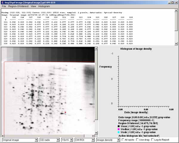
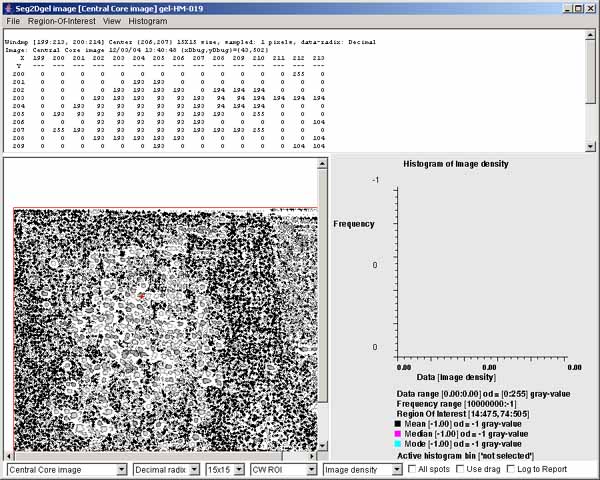
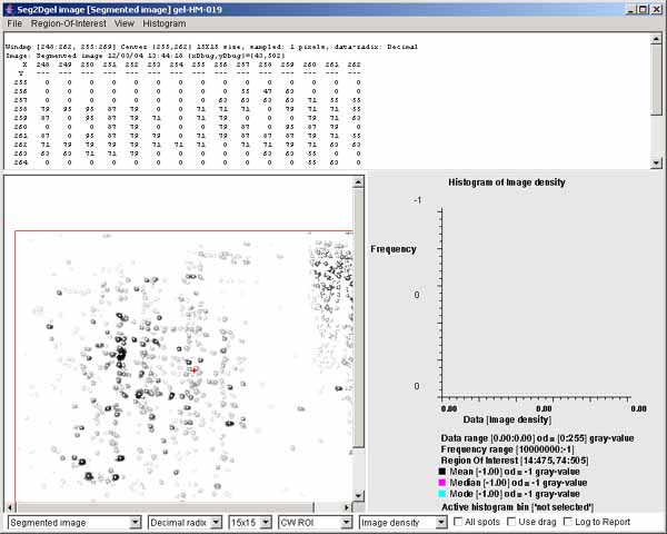
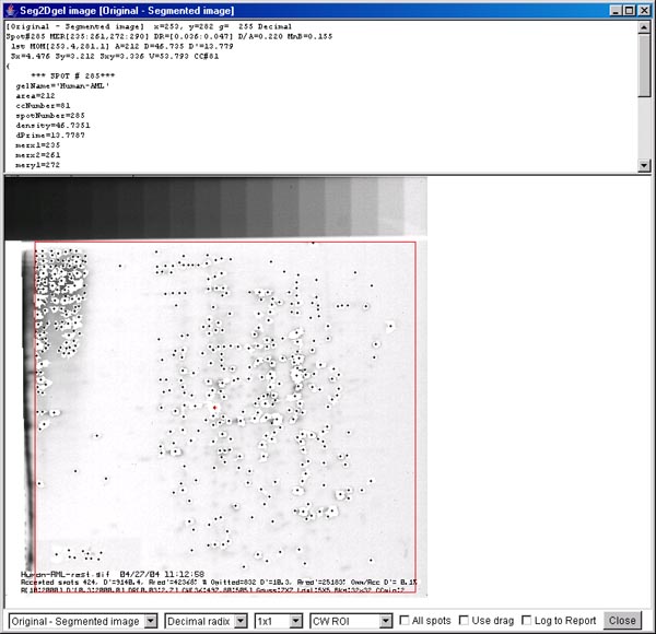