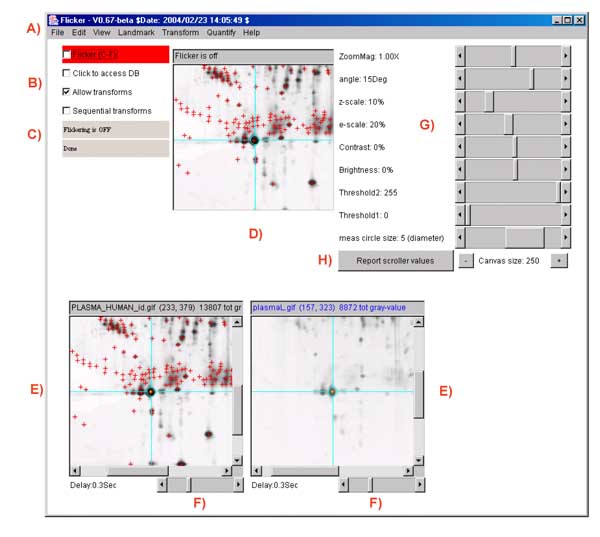
Figure.1 Screen view of the Flicker program This screen shot shows the pull-down menus (A) at the top of the Flicker window used to invoke file operations, editing, view selection, landmarking, image transforms, spot quantification, and help commands. A set of scroll bars on the right determines various parameters used in some of the transforms. The File menu options include opening new gel images. Checkboxes on the left (B) activate flickering and active gel map access if the data supports it. A set of status lines (C) appear below the checkboxes and indicate the state of operation and various other messages. The flicker image (D) is in the upper-middle of the frame when it is enabled. The two labeled human blood plasma gel images are shown in the bottom left and right scrollable image windows (E) that may be positioned to the region of interest. These windows also have associated flicker time-delays (F) used when flickering. Image plasmaH is an IPG non-linear gradient gel from SWISS-2DPAGE and plasmaL is a carrier-ampholyte linear gradient gel from the Merril Lab at NIMH. Transformed image results are shown in the same scrollable windows. The four checkboxes are: Flicker to enable/disable flickering; Click to access DB checkbox enables/disables access to a Web server that is associated with a clickable image DB if it exists for the selected image; Allow transforms checkbox enables/disables image transforms; Sequential transforms checkbox enables/disables using the last image transform output as input for the next image transform. Parameters are directly specified using sliders (G) to adjust zoom magnification, contrast, brightness, etc. A popup scrollable report window (not shown) logs all text output that appears in the status lines. You can popup the report window with the current scroller values by the Report scroller values button (H). This text may be saved to a text file on your local disk for printing or further analysis. The size of the three image canvases may be increased/decreased using the "+" / "-" buttons under the parameter scrollbars (H).
If it appears that a spot and the surrounding region do match, then
one has more confidence that the objects are the same. This putative
visual identification is our definition of matching when doing a
comparison. Full identification of protein spots requires further work
such as cutting spots out of the gels and subjecting them to sequence
analysis, amino-acid composition analysis, mass spectrometry, testing
them with monoclonal antibodies, or other methods.
Using the mouse, the user initially
selects (by clicking on the image - left or right window) what they
suspect is the same prominent spot or object in similar morphologic
regions in the two gel images. If you click on the spot with the
Control key pressed, it will center that image at that spot in
the window and also center it in the flicker window. You can
continuously adjust the position in the flicker window, without
changing the selected window position, by selecting the image you want
to recenter and draging the mosue. When these two local regions come
into alignment, they appear to pulse and the images appear to fuse
together. At this point, differences are more apparent and it is
fairly easy to see which spots or objects correspond, which are
different, and how they differ. We have found that the user should be
positioned fairly close to the flicker window on the screen to
optimize this image-fusion effect (i.e., it does not work as well
standing back more than a few feet from the screen).
Another useful trick is change the image canvas size after doing the
initial alignment. This may help you focus on a smaller region after
you have done the rough alignment. You can either use the "+" / "-" buttons under
the parameter scrollbars (Figure 1.I), or you can
use the Control-keypad + and Control-keypad - keys.
When comparing a light spot in one gel with the putative paired darker
spot in the other gel one may want to linger longer on the lighter
spot to make a more positive identification. Because of this, we give
the user the ability to set the display times independently for the
two images (typically in the range of 0.01 second to 1.0 second with a
default of 0.30 second) using separate Delay scroll bars
located under each image (Figure 1.E). If the
regions are complex and have a lot of variation, longer display times
may be useful for both images. Differential flicker delays with a
longer delay for the light gel are useful for comparing light and dark
sample gels. This lets you stare at the lighter spots to have more
verification that they are actually there.
These flicker delay values are saved for the left and right images
when you save the Flicker state.
In place of the Web browser, you can just have it report the
Swiss-Prot ID and the protein name annotation from the Swiss-2DPAGE
Web server. Set the (View |
The next discussion describes looking
up the (ID, protein names) for a set of spots you have defined.
If you then have a set of corresponding spots you have defined in your
gel, you can then edit their annotation so it matches the reference
gel that you just assigned putative spot identifications. This is
described in the following Figures 3.1a through 3.1d You
can lookup the protein (ID,names) for a set of spots you have defined
in the active gel map image that is link to federated 2D gel
databases. See the vignettes for query a spot's putative
identity and assigning a spot's
putative identity for more details.
An additional option that makes this easier to use is to enable the
(Edit |
Some of these transforms involve spatial warping, which maps a local
region of one image onto the geometry of the local region of another
image while preserving its grayscale values. Another useful operation
is contrast enhancement that helps when comparing light or dark
regions by adjusting the dynamic range of image data to the dynamic
range of the computer display. Figure 2
shows the effects of contrast adjustment. Other transforms include
image sharpening and contrast enhancement. Image sharpening is
performed using edge enhancement techniques such as adding a
percentage of the gradient or Laplacian edge detection functions to
the original grayscale image. The gradient and Laplacian have higher
values at the edges of objects. In all cases, the transformed image
replaces the image previously displayed. Flicker will normally
transform the input imate to an output image. You can use another
transform on the previously transformed image if you had set the
b)
c)
In both systems, you can specify additional command line arguments in
Windows .bat and unix .sh scripts below.
If you have your own gels (JPEG, GIF or TIFF formats), you can try
loading them. You may want to limit resolution by first decreasing
their size using an image editing program like Adobe PhotoShop or the
shareware program ThumbsPlus (www.cerious.org ). Large very high
resolution images that are 20Mb to 40Mb will not work as well. We
suggest reducing the size to about 1Kx1K for good interactivity if you
have any problems with running out of memory or very sluggish
response. These image editing programs can also be used for converting
other formats to JPEG, GIF or TIFF formats that Flicker can read.
An Internet connection is required to download the program from the
Flicker Web site. New versions of the program and associated demo data
will become available on this Web site and can be uploaded to your computer using the various
(File | Update | ...) menu commands. If you have obtained the
installer software that someone else downloaded and gave to you, then
you do not need the Internet connection to install the program. If you
will be using the active gel image maps associated with federated
2D-gel databases, then you will need the Internet connection for
accessing those databases. You do not need the Internet for local
image comparisons.
If you are using the Windows Flicker.exe file to start the program
or clicking on the Flicker.jar file, you can't change the default
startup memory.
If you are using the Flicker.jar in a script using the java interpreter
as in the following example which uses the -Xmx96M
(specifying using 96 at startup). Change 96 to a larger size
if you want to increase startup memory.
For example, if you have four images image1, image2, image3
and image4 in your directory MyData-folder, then the
submenu entries will be
Note that it does not generate comparisons between
directories. You can still do that by clicking on the left (and then
later the right) image and using the (File | Open image file)
command to manually load the file into the image. If you want to do
this often, put your images in the same directory.
If you have this type of data, it will also add the (File | Open
user images | List user's images by directory) command. You
can use this to get a report of all of the files in the popup report
window.
You will not use the (Files | Update | Flicker program)
command. Using this command will get the latest release which is not
what you want if you want an earlier release.
Instead do the following. You copy the version of
Flicker.jar you want to the location on your disk where you
had installed Flicker overwriting the previous version. For example,
on MS Windows this is typically
There are a number of .jar files of the form
To be used with the Flicker startup process, this file must be
called Flicker.jar, so you must rename it as Flicker.jar.
The procedure is as follows:
Once you are sure your remote web site is set up correctly, then
simply use the (File | Update | Add user's Flicker Demo Images DB
by URL) command to download and and update the Flicker demo
database. After it is successful, it will tell you to exit and restart
Flicker. If you go to the Files | Open demo images| ... menu,
you should see the new demo data you have installed.
The Flicker.properties file is the user-specific preferences
for generic properties such as colors, view options, etc. This file is
created when you exit flicker and read (if it exists) when you start
it. If you have never run flicker or the file was deleted, Flicker
uses the default values. If the Flicker.properties file exists,
it overides these files. If you have started Flicker using a .flk
startup file, this in turn overides any settings from the
Flicker.properties file.
For example, you may want to use a red trial object cursor instead of
yellow, etc. If you have both a Flicker.properties file and
are starting Flicker using a .flk startup file, it (1) reads the user
preferences first from Flicker.properties, and then (2) reads
the .flk startup file to overide these preferences. If you want to
reset the standard view, use the (Edit | Reset default view)
command to overide the previous view read from
Flicker.properties. If the you ever have problems starting
Flicker because of a corrupted Flicker.properties file, just
delete it (it is kept in the same directory where you installed
Flicker) and restart Flicker. When you exit, it will create a new
properties file.
In the mean time, we refer to "density" as either of these two
measurements. You may measure the total integrated density (summing
the pixel gray values or OD), or mean density (the total
density/#pixels in the region). This background density is used to
correct the measurement density if it was defined (otherwise 0.0 is
assumed). Note that you may clear the background measurement circle
using the (C-W) command.
You can save the spot list in a tab-delimited file suitable for import
to Excel, by 1) clearing the Popup Report Window; 2) select the image
you want and use (Quantify | Measure by circle | List spots in the
spot list (tab-delimited)) command; 3) then, Save the text in the
Popup Report Window or cut and paste it into Excel, etc.
It is possible to generate a list of paired spots between the two
images using the (Quantify | Measure by Circle | List paired 'id'
annotated-spots in both spot lists (tab-delimited)) command. It
lists paired spots that occur in the spot lists of both gels and have
the same annotation 'id' values (case-sensitive). The user assigns
the spot 'id' annotations using the (C-I) spot editing command
to assign the case-sensitive spot identifiers. (C-E) command may
also be used to edit the ids'. The paired spot data list may be
exported to Excel similar to what was described in the last paragraph
for spot lists.
Note that the background density is not the same everywhere on
the gel image. Therefore if you are measuring spots in regions of the
gel with quite different background (e.g., tail streaks from other
spots, etc.), to get better estimated quantification you need to
redefine the background adjacent to where you are making
measurements. Recent versions of Flicker track the most recent
background (C-B) estimate and associate it with new measured
spots (C-M) until you redefine it.
Figures 12a-12h show various permuations of the spot list overlay
options. Figure 13 shows an example of a histogram of the Region Of
Interest (ROI). Figure 14 shows examples of calibrating gray scale a step
wedge scanned with the image using the step wedge calibration
wizard. Figure 15 shows calibrating grayscale where there are
calibration spots in the image by using the spot list calibration
wizard.
Panels (a.1) and (a.2) show a single spot measurement
image and report and does not create a list of measured spots. The
(Quantify |
Once an image is calibrated and the calibration saved (in the
{installation directory}/cal/{imageFile}.cal file), it may be
reused everytime the image is loaded into Flicker. The initial
calibration is created from the step wedge data and known
corresponding OD values using a histogram specified by a region of
interest (ROI) specified as the step wedge region.
To make it easier to demonstrate this process, we have set up special
demo calibration data for the four demo Leukemia gels. If you have
enabled (Quantify | Calibration | Use demo leukemia gels ND wedge
calibration preloads) checkbox, it will preload the OD values and
step-wedge ROI for demonstration purposes. If you are using any other
data, you must specify the OD values and step-wedge ROI. You invoke
the wizard by the (Quantify | Calibration | Optical density by step
wedge) command. This will popup the calibration wizard window.
You may also list the saved spots in the report window (shown in
Figure 16b). Hint, press the Clear button in the report window
first. Note that if you save the flicker state, then the spot lists
will be saved in the .flk file state and associated .spt spot list
files in the spt/ directory. Flicker will restore the spot
lists if you start flicker on the saved .flk startup file.
Flicker can then use the annotated spot lists you have generated to
create a paired spot table shown below.
As part of the demonstrations, we present a series of as short vignettes that have
answers to specific "How do I do ...?" types of questions. There are
several demonstration images that are available when you download and
install Flicker. Look in the (File | Open demo images)
menu. These commands will load pairs of demonstration images.
1. Flickering gel images
The basic concept of using flickering as a dynamic visualization
technique is simple. If two images may be perfectly aligned then one
could simply align them by overlaying one over the other and shifting
one image until they line up. However, many images such as 2D PAGE
gels have rubber-sheet distortion (i.e., local translation, rotation,
and magnification - linear over short distances and non-linear over
the entire gel). This means there is more distortion in some parts of
the image than in others. Although it is often impossible to align the
two whole images at one time, they may be locally aligned
piece-by-piece by matching the morphology of local regions.1.1 Flickering
When flickering two images with the computer, one aligns putative
corresponding subregions of the two rapidly alternating images. The
flicker window overlays the same space on the screen with the two
images and is aligned by interactively moving one image relative to
the other using the cursor in either or both of the lower
images. Enable the Flicker checkbox (Figure
1.B) to turn on flickering and disable it to shut it off.1.2 Selecting the proper time delays when flickering
The proper flicker delays, or time each image is displayed on the
screen, is critical for the optimal visual integration of image
differences. We have also found that optimal flicker rates are
dependent on a wide variety of factors including: amount of
distortion, similarity of corresponding subregions, complexity and
contrast of each image, phosphor decay time of the display, ambient
light, distance from the display, individual viewer differences,
etc. We have found the process of flickering images is easier for some
people than for others.1.3 Mouse control of images
The following mouse and key-modified mouse operations control various
actions.
![]() Click to access DB
was enabled, it
will try to locate that spot in the associate Web server for that
image (see Figure 2).
Click to access DB
was enabled, it
will try to locate that spot in the associate Web server for that
image (see Figure 2).
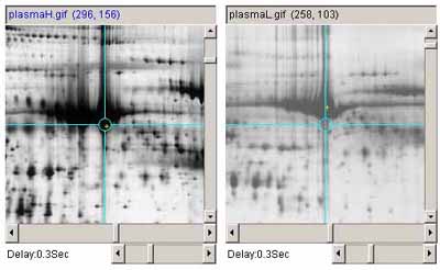
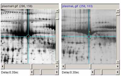
Figure 2. Example of adjusting the image contrast on one image to
match the overall contrast of the other. A)
shows the original plasmaH and PlasmaL images before contrast
adjustment b) shows the plasma images after the contrast was
adjusted in the plasmaL image.
1.4 Lookup of putative spot identification on Swiss-2DPAGE
Protein spots may be putatively identified using active map images
that link to federated 2D gel databases such as SWISS-2DPAGE. First, load an
active map image for your type of biological material (if it can be
found). Then flicker align the two gels around the spot(s) you are
interested in. Then enable the ![]() Click to access DB checkbox. Then
set the (View |
Click to access DB checkbox. Then
set the (View | ![]() Use protein DB
browser, else lookup ID and name on active images) menu checkbox
command is enabled. Finally, click on the spot of interest and this
brings up the specific protein
annotation page from the active DB server (in this case
SWISS-2DPAGE) in a Web browser. Figure 3
shows an illustration of procedure.
Use protein DB
browser, else lookup ID and name on active images) menu checkbox
command is enabled. Finally, click on the spot of interest and this
brings up the specific protein
annotation page from the active DB server (in this case
SWISS-2DPAGE) in a Web browser. Figure 3
shows an illustration of procedure.![]() Use
protein DB browser, else lookup ID and name on active images) menu
checkbox command is disabled. Then when you click on a spot, it will
now try to get the Swiss-Prot ID and the protein name by the spot's
coordinates and display the results in your report window.
Use
protein DB browser, else lookup ID and name on active images) menu
checkbox command is disabled. Then when you click on a spot, it will
now try to get the Swiss-Prot ID and the protein name by the spot's
coordinates and display the results in your report window.

Figure 3. Protein spots may be putatively identified using active
map images that link to federated 2D gel databases.
First, load an active map image for you type of biological material
(if it can be found). Then flicker align the two gels around the
spot(s) you are interested in. Then enable the ![]() Click to access DB
checkbox. Finally, click on the spot of interest and this brings up
the Web page from the active DB server (in this case SWISS-2DPAGE).
If the (View |
Click to access DB
checkbox. Finally, click on the spot of interest and this brings up
the Web page from the active DB server (in this case SWISS-2DPAGE).
If the (View | ![]() Use protein DB
browser, else lookup ID and name on active images) is enabled,
then clicking on a spot will popup a Web browser with the associated
database page (as is shown). If the checkbox is off, then it will get
the data from that web page and report it. If you have defined a set
of spots in a spot list in an active gel, the (Quantify | Measure
by Circle | Lookup Protein IDs and Names from active map server
(selected image)) menu command will try to lookup each spot in the
list by its coordinates and will save the results (Swiss-Prot ID and
protein name) as the spot annotation's (id,name).
Use protein DB
browser, else lookup ID and name on active images) is enabled,
then clicking on a spot will popup a Web browser with the associated
database page (as is shown). If the checkbox is off, then it will get
the data from that web page and report it. If you have defined a set
of spots in a spot list in an active gel, the (Quantify | Measure
by Circle | Lookup Protein IDs and Names from active map server
(selected image)) menu command will try to lookup each spot in the
list by its coordinates and will save the results (Swiss-Prot ID and
protein name) as the spot annotation's (id,name).
1.4.1 Looking up and assigning putative spot IDs for lists of spots
If you have defined a set of spots in a spot list for an active gel,
the (Quantify | Measure by Circle | Lookup Protein IDs and Names
from active map server (selected image)) menu command will try to
lookup each spot in the list by its coordinates and will save the
results (Swiss-Prot ID and protein name) as the spot annotation's
(id,name). Note that you must be connected to the Internet. After this
lookup has finished (it may take a while), use the (Quantify |
Measure by Circle | List spots in the spot list for selected
image) to view the filled in table. The (C-Q) key-command
may be use to stop the lookup procedure for a long list of spots after
it finishes the current spot lookup.
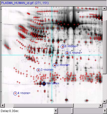
Figure 3.1a) First define a set of spots in the active
gel (described under the Quantify menu).
You might want to view the spot annotations by setting the (View |
Set view measurement options | ![]() Use
'spot identifier ' for spot annotations) menu checkbox. Then
enable the
Use
'spot identifier ' for spot annotations) menu checkbox. Then
enable the ![]() Click to access DB
checkbox. Then, if you are connected to the Internet, with the active
gel selected, use the (Quantify | Measure by Circle | Lookup
Protein IDs and Names from active map server (selected image))
menu command. This will try to lookup each spot in the list by its
coordinates and will save the results (Swiss-Prot ID and protein name)
in each the spots annotation's (id,name).
Click to access DB
checkbox. Then, if you are connected to the Internet, with the active
gel selected, use the (Quantify | Measure by Circle | Lookup
Protein IDs and Names from active map server (selected image))
menu command. This will try to lookup each spot in the list by its
coordinates and will save the results (Swiss-Prot ID and protein name)
in each the spots annotation's (id,name).
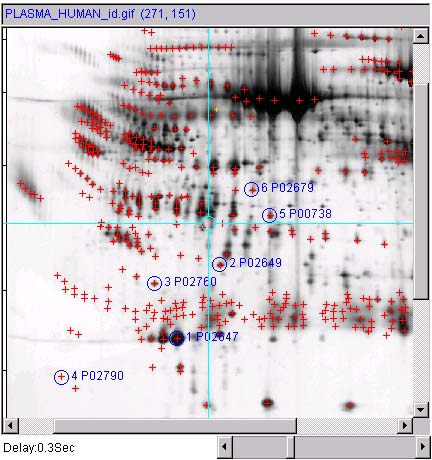
Figure 3.1b) Shows the updated spot list after the spots have
been identified from the active reference gel database. Now disable the ![]() Click to
access DB checkbox so that it does not popup the Web browser when
you then click on the image.
Click to
access DB checkbox so that it does not popup the Web browser when
you then click on the image.
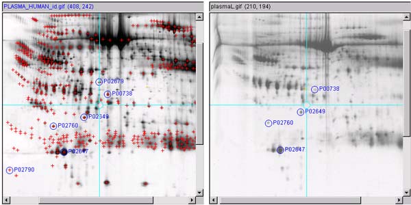
Figure 3.1 c) Then define a list of spots in the other
user gel by selecting the spot and typing (C-M). Repeat the following for each spot in the gel lists. First
select a spot in the reference gel, and then select the corresponding
spot in the user gel. Assign the same annotation to both by typing
(C-I).

Figure 3.1 d) This will popup "Edit spot annotation"
window with the spot identifier from the reference gel.
Just press the Done button and the annotation will be assigned to the
user gel spot you are editing.1.4.2 Accessing PIR UniProt, iProClass and iProLink server Web pages for selected proteins
You may optionally access PIR UniProt, iProClass and iProLink server Web
pages for selected proteins in the spot list through their Swiss-Prot
accession names. This is accomplished in a two-step process enabled
using the (Edit | Select access to active DB server | ![]() ...) checkbox command. You may select
either SWISS-2DPAGE, UniProt, iProClass or iProLink servers - or none
of these. If you measure a spot (select a spot in an active image and
then type C-M) (and are connected to the Internet), it will
also lookup the Swiss-Prot protein (accession name, and protein id) on
the SWISS-2DPAGE server. Then, if you enable "Click to access DB", it
will pop up the particular active DB server you have selected. Figures
3.2a UniProt,
3.2b iProClass, and
3.2c iProLink.
...) checkbox command. You may select
either SWISS-2DPAGE, UniProt, iProClass or iProLink servers - or none
of these. If you measure a spot (select a spot in an active image and
then type C-M) (and are connected to the Internet), it will
also lookup the Swiss-Prot protein (accession name, and protein id) on
the SWISS-2DPAGE server. Then, if you enable "Click to access DB", it
will pop up the particular active DB server you have selected. Figures
3.2a UniProt,
3.2b iProClass, and
3.2c iProLink.![]() Auto measure, protein
lookup and Web page popup) checkbox command. Then when you click
on a spot in an active image (associated with a Web database), it
will: 1) measure the spot and add it to the spot list; 2) lookup the
Swiss-Prot (name, id); and 3) pop up the Web server on the currently
selected active DB server.
Auto measure, protein
lookup and Web page popup) checkbox command. Then when you click
on a spot in an active image (associated with a Web database), it
will: 1) measure the spot and add it to the spot list; 2) lookup the
Swiss-Prot (name, id); and 3) pop up the Web server on the currently
selected active DB server.
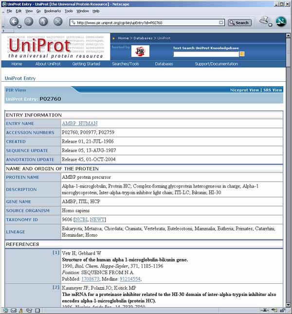
Figure 3.2a) Results of accessing PIR UniProt server Web pages for
protein 3 P02760 from Figure 3.1b. This was
accessed using the method describe in section 1.4.2 above by enabling
(Edit | Select access to active DB server | ![]() Use PIR UniProt DB access) checkbox
command set, enabling (Edit |
Use PIR UniProt DB access) checkbox
command set, enabling (Edit | ![]() Auto
measure, protein lookup and Web page popup) checkbox command, and
then clicking on the spot.
Auto
measure, protein lookup and Web page popup) checkbox command, and
then clicking on the spot.
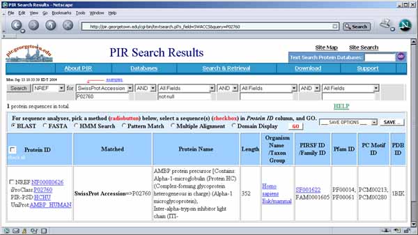
Figure 3.2b) Results of accessing PIR iProClass server Web
pages for protein 3 P02760 from Figure 3.1b. This
was accessed using the method describe in section 1.4.2 above by
enabling (Edit | Select access to active DB server | ![]() Use PIR iProClass DB access) checkbox
command set, enabling (Edit |
Use PIR iProClass DB access) checkbox
command set, enabling (Edit | ![]() Auto
measure, protein lookup and Web page popup) checkbox command, and
then clicking on the spot.
Auto
measure, protein lookup and Web page popup) checkbox command, and
then clicking on the spot.
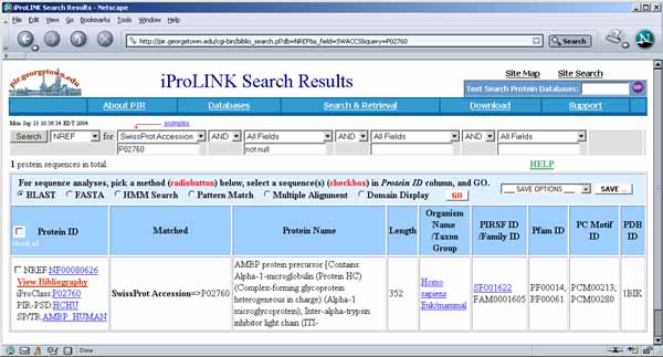
Figure 3.2c) Results of accessing PIR iProLink server Web
pages for protein 3 P02760 from Figure 3.1b. This
was accessed using the method describe in section 1.4.2 above by
enabling (Edit | Select access to active DB server | ![]() Use PIR iProLink DB access) checkbox
command set, enabling (Edit |
Use PIR iProLink DB access) checkbox
command set, enabling (Edit | ![]() Auto
measure, protein lookup and Web page popup) checkbox command, and
then clicking on the spot.
Auto
measure, protein lookup and Web page popup) checkbox command, and
then clicking on the spot. 1.5 Checkbox control of flickering and database access
There are four checkboxes in the upper left part of the window (Figure 1.B) that control commonly used
options. Figure 3 describes these options in more detail.
![]() Flicker (C-F) checkbox enables/disables flickering.
Flicker (C-F) checkbox enables/disables flickering.
![]() Click to access DB checkbox enables/disables access to a
Web database server that is associated with a clickable image - if it
exists for the selected image. Turning on this option will disable
flickering.
Click to access DB checkbox enables/disables access to a
Web database server that is associated with a clickable image - if it
exists for the selected image. Turning on this option will disable
flickering.
![]() Allow transforms checkbox enables/disables image transforms
Allow transforms checkbox enables/disables image transforms
![]() Sequential transforms
checkbox enables/disables using the last image transform output as
input for the next image transform (image composition) if the
Sequential transforms
checkbox enables/disables using the last image transform output as
input for the next image transform (image composition) if the ![]() Allow transforms is enabled
Allow transforms is enabled
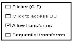
Figure 4. Screen view of the Flicker checkbox controls. This shows the global checkbox controls that are used to set
operational modes for flickering, Web database access and image
processing transforms. These values are saved when you save the
Flicker state.
2. Image enhancement prior to flickering - Transforms
It is well-known that 2D gels often suffer from local geometric
distortions making perfect overlay impossible. Therefore, making the
images locally morphologically similar while preserving their
grayscale data may make them easier to compare. Even when the image
subregions are well aligned, it is still sometimes difficult to
compare images that are quite different. Enhancing the images using
various image transforms before flickering may also help. The
Transforms menu contains a number of image transforms. Click on
the image you want to transform and then select the transform
from the list of available transforms. If you select neither the left
or right image, it will perform the transform on both images.![]() Sequential transforms checkbox.
Sequential transforms checkbox.2.1 Display models for image transform and brightness-contrast
operations
There are several display models for combinations of using image
transforms and brightness contrast or zoom filtering. These are
applied to the left and right windows and also are shown in the
flicker window. Two checkboxes in the upper left of the main window
control transforms: ![]() Allow
transform enables/disables transforms, and
Allow
transform enables/disables transforms, and ![]() Sequential transforms allows using
the previous transform as the input to the next transform, i.e., image
composition. The original image is denoted iImg. If you allow
transforms and are also composing image transforms, you may optionally
use the previous transformed output image (denoted oImg) as
input to the next image transform. The output (either iImg or
oImg) is then sent to the output1. Then the output2 which is
either zoomed or not is sent to the brightness-contrast filter if
active (specified by dragging the mouse in the selected window with
the SHIFT-key pressed). The output2 of the brightness-contrast
filter is denoted as bcImg. If you have never used the zoom or
brightness-contrast filtering since loading an image, then zImg
and bgImg are not generated and hence not used in the displayed
image. Figure 5. illustrates these four cases.
Sequential transforms allows using
the previous transform as the input to the next transform, i.e., image
composition. The original image is denoted iImg. If you allow
transforms and are also composing image transforms, you may optionally
use the previous transformed output image (denoted oImg) as
input to the next image transform. The output (either iImg or
oImg) is then sent to the output1. Then the output2 which is
either zoomed or not is sent to the brightness-contrast filter if
active (specified by dragging the mouse in the selected window with
the SHIFT-key pressed). The output2 of the brightness-contrast
filter is denoted as bcImg. If you have never used the zoom or
brightness-contrast filtering since loading an image, then zImg
and bgImg are not generated and hence not used in the displayed
image. Figure 5. illustrates these four cases.
 a) If no transforms or brightness-contrast filtering is used
    on the selected image
                   (No transforms)
        iImg -----------------------------------> output1

 b) Image transforms may be composed from the original image (iImg) or
    from Sequential composition of image transforms on the
    selected image
                   (optional sequential)
                  +----------------------+
                  |                      |
                  V                      |
        iImg -----> Transform -----------> oImg --> output1

  c) The image may be optionally zoomed if the magnification is not 1.0X
     on the selected image
                 (zoom)
        output1 --------> zImg ------------> output2
     or
                 (No zoom)
        output1 ---------------------------> output2


  d) Using brightness-contrast filter on output image
                 (BC filter)
        output2 -----------------> bcImg --> display
     or
                 (No BC filter)
        output2 ---------------------------> display
Figure 5. Output image as a function of image processing modes.
This shows the four modes that create an output image
depending on whether the brightness-contrast processing is used and if
image transforms are used. The (File Reset images) menu command
resets the display processors to the initial state (a).
2.2 Keyboard menu shortcut controls
There are several menu short-cut key combinations that may be used to
perform operations instead of selecting the command from the pull-down
menus. The command short-cut notation C-key means to
hold the Control key and then press the specified key.
![]() Flicker (C-F))
Flicker (C-F))
2.3 Sliders for defining transform parameters
The set of parameter sliders are in the upper right part of the window
(Figure 1.G and Figure 6)
are used for adjusting parameters for the various image transforms
(see Transform menu). The size of the
three image canvases may be increased/decreased using the "+" / "-" buttons under
the parameter scrollbars. The current canvas size for the three image
windows is displayed (in pixels).
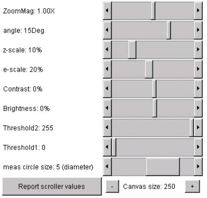
Figure 6. Screen view of the Flicker parameter slider controls.
This screen shot shows the parameter slider control
that are used to set parameters for the various transforms. Separate
parameter values are assigned to the left and right windows and are
saved when you save the Flicker state. Pressing the Report scroller
values button will popup the report window and display the current
parameter values for both the left and right windows. The size of the
three image canvases may be increased/decreased by pressing the
"+" / "-"
buttons under the parameter scrollbars. The current canvas size for
the three is displayed (in pixels).
2.4 Example of changing image magnfication
Sometimes when comparing gels from different sources, you want want to
change the magnification of one of them so they are easier to compare.
Figure 7 shows an example of adjusting the
magnification of the selected image by 1X, 2X and 0.5X using the zoom
mag slider.
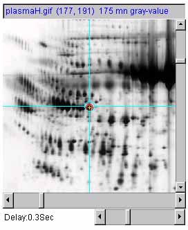
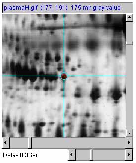
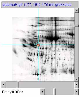
Figure 7 shows an example of adjusting the magnification of the
selected image by 1X, 2X and 0.5X using the zoom mag slider. a) is the original image at 1.0X zoom. b) is
the original image at 2.0X zoom. c) is the original image at
0.5X (de)zoom.
3. Reporting the status in the popup status window
The Flicker status information is displayed in several places.
![]() Display gray values (C-G)) option. It
reports the total measurement circle density if the (Quantify |
Display gray values (C-G)) option. It
reports the total measurement circle density if the (Quantify |
![]() Use sum density else mean
density)) option is enabled.
Use sum density else mean
density)) option is enabled.
a) 

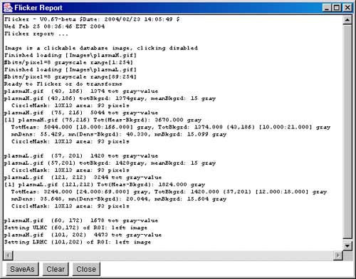
Figure 8. Screen view of the popup information windows. a) Flicker Yes/No/Cancel window to give you a chance
to save data that you have edited or created. b) Flicker error or
warning alert window when illegal conditions occur. c) Flicker
Report window This screen shot shows the popup report window that
contains a log of all activity. You can save this window's contents or
clear it. If you close the window, it continues to log activity and
may be popped up again using the (View | ![]() Show report popup) command or the
Report scroller values button underneath the parameter
scrollers.
Show report popup) command or the
Report scroller values button underneath the parameter
scrollers.
4. Downloading, installing and running Flicker
The following method can be used todownload the
Zipped Flicker-dist
and install it as described below. This includes a
launch4j windows installer.4.1 Downloading and installing Flicker
The installation packages are now available from the
Files mirror under the Flicker releases. Look for the most recent release named
"Flicker-V.XX.XX-dist.zip". These include the program, required jar libraries,
demo data, Windows batch and Unix shell scripts. Download the zip file and put the
contents where you want to install the program. Note that there is a Flicker.exe
(for Windows program). You might make a short-cut to this to use in more easily
starting the program. Alternatively, you can use the sample .bat and .sh scripts
to run the program explicitly via the java interpreter. Note that this method
assumes that you have Java installed on your computer and that it is at least
JDK (Java Development Kit) or JRE (Java Runtime Environment) version 1.5.0.
If you don't have this, you can download the latest version free from the
java.sun.com Website.
4.2 Downloading and installing Flicker
The following is a short procedure that is suggested for downloading
and installing Flicker.
4.3 Starting Flicker
There are several ways to run the program. On Windows, you can start
Flicker by clicking on the startup icon shown in Figure 10 below.
For Unix systems including MacOS-X, you can start Flicker from
the command line by running the Flicker.jar file. If your computer is setup
to execute jar files, just type the jar file. Normally it
comes up with the two demonstration human plasma 2D-gel images
(plasmaH.gif - an IPG gel from SWISS-2DPAGE on the left) and
(plasmaL.gif - a carrier ampholyte gel from Dr. Carl Merril/NIMH on
the right).
REM File: Flicker-startup.bat
REM Simple Flicker batch script for Windows.
REM Starts Flicker from its jar file  on the command line.
REM To use more memory on startup, increase 96 (Mbytes) to a larger value.

java -Xmx96M -jar Flicker.jar
and
#!/bin/sh
# File: Flicker-startup.sh
# Simple Flicker batch script for Unix.
# Starts Flicker from its jar file  on the command line.
# To use more memory on startup, increase 96 (Mbytes) to a larger value.

java -Xmx96M -jar Flicker.jar
![]()
Figure 10. Startup icon for Flicker. This is
installed on your computer (default is the desktop) when you install
Flicker. Clicking on the icon starts Flicker. When you (File |
SaveAs state file) to save the state of your session with the gels
you have loaded, it will let you name the .flk startup file. You then
can reload the state using the (File | Open state file) to
restore the state.
4.4 Requirements: minimum hardware and software requirements
A Windows PC, MacIntosh with MacOS-X, a Linux computer or a Sun
Solaris computer having a display resolution of at least
1024x768. We find that a 1024x768 is adequate, but a 1280x1024 screen
size much better since you can make the flicker windows larger and see
the Popup Report window at the same time. At least 30 Mb of memory
available for the application is required and more is desirable for
comparing large images or performing transforms. If there is not
enough memory, it will be unable to load the images, the transforms
may crash the program or other problems may occur.Increasing or decreasing the allowable memory used by Flicker
You may increase memory by adjusting the startup .bat or .sh shell
startup scripts. For very large images you could set it to 512 mb or more
if your computer has at least that much memory. The allowable memory
range you may set it to is 30 Mb to 1768 Mb. If you are working with
very large images that require a lot of memory, you might want to
increase the memory available at startup.
java -Xmx96M -jar Flicker.jar {additional command line args}
4.5 Files included in the download
The following files are packaged in the distribution and installed
when you download and install Flicker from
the Web server.
4.6 Local (Flk...DB.txt) database files
When Flicker is installed, several tab-delimited (spreadheet derived
with column names) .txt files are available in the DB/
directory (located where the Flicker.jar file is
installed). These DB/Flk*DB.txt files are read on startup and
are used to setup the (File | Open ... image | ...) menu trees.
4.7 Local Folders and files created and used by Flicker
When Flicker is first started, it will check for the following folders
and files in the installation directory and create them if they can
not be found.
4.8 Adding your own image data to the user Images/ database
There is another way for users to add many of their gel images without
editing the DB/FlkDemoDB.txt file. When you place your image
data directories in the Images/ directory, Flicker will
discover them when it starts and add them to the demo menu. It works
as follows:
4.8.1 Example of pairs of images
An example of the (File | Open user images | Pairs of images |
...) may help clarify this.
![]()
4.9 Updating the latest versions of the program and data from the
Web server
You can update your program and active image map and demo image data
files using the various Update options in the Files menu. The (File
| Update | Flicker program) command downloads and installs the
latest Flicker.jar file. The (File | Update | Active Web Maps
DB) command downloads and installs the latest active Web maps
database DB/FlkMapDB.txt file. The active maps point to federated
2D-gel web servers with identified spots. The (File | Update |
Demo images DB) command downloads the latest demo images and the
DB/FlkDemoDB.txt file.4.9.1 Instructions for using an older version of Flicker
The version of flicker you use is dependent on the version
of the Flicker.jar file.
C:\Program Files\Flicker\Flicker.jar
If you installed Flicker elsewhere on your computer, then that is
where you need to change it. Go to the files distribution in the File
mirror web page.
Flicker.jar-V0.xx
Copy the one you want to your computer.
4.9.2 Adding your own or another Web sites demo data to your
Flicker Demo database
You can add set set of demo gel data to the Flicker demo database from
any Flicker demo-data compatible web site. This data must be is
exactly the form required that is spelled out in this manual (see Section 4.3 details on FlkDemoDB file
formats. Once you have confirmed that the Web site is compatible,
it is simple to add that data to your local Demo database. If the Web
site data changes, when you do the update, it will replace existing
entries with the new data from that Web site. NOTE: all file names are
case-dependent so becareful when building your DB/ tables and
in naming the images. The Web site should have 2 folders:
   DB/
and
   Images/
The DB/ folder must have two files FlkDemoDB.dir (the
list image images in the Images/ folder, and
FlkDemoDB.txt which is a tab-delimited spread sheet describing
the demo images. NOTE: demo images generally live in the top level of
the Images/ directory. They are not in subdirectories of the
Images/ directory. If you are designing such a remote demo
Web site, you could model the files from the current Flicker DB
files.5. Saving and restoring the Flicker state
Flicker gives you the option of saving the current state of your
session including the images your are looking at and the parameter
values of the sliders, etc. To save the current state, use the
(File | Save (or SaveAs) state file) command. This creates a
file with a .flk file extension in the installation
FlkStartups/ folder (default DB/FlkStartup.flk).
Any time while running Flicker, you can also use
(File | Open state file) command to change it to another
saved Flicker state.
6. Pull-down menus
The menu bar commands are divided into menus divided by function.
Menu notation
In the following menus, selections that are sub-menus are
indicated by a '![]() '. Selections prefaced with a '
'. Selections prefaced with a '![]() ' and indicate '
' and indicate '![]() ' indicate that the command is a checkbox
that is enabled and disabled respectively. Selections prefaced with a
'
' indicate that the command is a checkbox
that is enabled and disabled respectively. Selections prefaced with a
'![]() ' and indicate '
' and indicate '![]() ' indicate that the command is a
multiple choice "radio button" that is enabled and disabled
respectively, and that only one member of the group is allowed to be
on at a time. The default values set for an initial database are shown
in the menus. Selections that are not currently available will be
grayed out in the menus of the running program. The command short-cut
notation C-key means to hold the Control key and then
press the specified key.
' indicate that the command is a
multiple choice "radio button" that is enabled and disabled
respectively, and that only one member of the group is allowed to be
on at a time. The default values set for an initial database are shown
in the menus. Selections that are not currently available will be
grayed out in the menus of the running program. The command short-cut
notation C-key means to hold the Control key and then
press the specified key.
6.1 File menu
These commands are used to load/save the Flicker .flk state, load
images, active map URLs, update (from the server) program,
DB/Flk*DB.txt database files, demo images, and user's
images. It also saves and restores the Flicker state, does updates
from the server. You can save transformed or overlay images as GIF
files in the tmp/ directory.
![]() - load pairs of
demonstration gel images
- load pairs of
demonstration gel images
![]() - load single
(selected image) or pairs of user's image data if they had set
up the Images/ directory as
specified on their data
- load single
(selected image) or pairs of user's image data if they had set
up the Images/ directory as
specified on their data
![]() - load active gel
image from the Internet in selected image
- load active gel
image from the Internet in selected image
------------------------------------
------------------------------------
![]() - update Flicker
programs and data from open2dprot.sourceforge.net/Flicker
server
- update Flicker
programs and data from open2dprot.sourceforge.net/Flicker
server
------------------------------------
------------------------------------
6.2 Edit menu
These commands are used to change various defaults. These are saved
when you save the state and when you exit the program.
![]() - change the size
of the 3 canvases and the overall Flicker window
- change the size
of the 3 canvases and the overall Flicker window
![]() - change overlay
graphics colors
- change overlay
graphics colors
![]() -
to change the target color
-
to change the target color
![]() -
to change the trial object color
-
to change the trial object color
![]() -
to change the landmarks color
-
to change the landmarks color
![]() -
to change the circle mask measurement color
-
to change the circle mask measurement color
![]() -
to change the image guard region color
-
to change the image guard region color
------------------------------------
![]() Use linear else log of TIFF files > 8-bits - transform
the input TIFF image if it is more than 8-bits of intensity.
Use linear else log of TIFF files > 8-bits - transform
the input TIFF image if it is more than 8-bits of intensity.
![]() Enable saving transformed images when do a 'Save(As)
state' - If you have transformed the left and/or the right
image(s) and are allowing transforms, then this will save the
transformed images in a tmp/ directory as .gif files
when you save the Flicker state.
Enable saving transformed images when do a 'Save(As)
state' - If you have transformed the left and/or the right
image(s) and are allowing transforms, then this will save the
transformed images in a tmp/ directory as .gif files
when you save the Flicker state.
![]() Use protein DB browser, else lookup ID and name on active
images - used when click on a spot in an active DB that has
Use protein DB browser, else lookup ID and name on active
images - used when click on a spot in an active DB that has
![]() click to access DB
checkbox enabled. If this command is set, report the protein
identication in a popup window. If it is not set, then lookup
the protein ID and name and report it in the popup Report window.
click to access DB
checkbox enabled. If this command is set, report the protein
identication in a popup window. If it is not set, then lookup
the protein ID and name and report it in the popup Report window.
------------------------------------
![]() Auto measure, protein
lookup and Web page popup - if one the following active DB
servers is enabled, it will: 1. measure the spot and add it to
the spot list; 2. lookup the Swiss-Prot (name, id); and 3. pop
up the Web server on the currently selected active DB server.
Auto measure, protein
lookup and Web page popup - if one the following active DB
servers is enabled, it will: 1. measure the spot and add it to
the spot list; 2. lookup the Swiss-Prot (name, id); and 3. pop
up the Web server on the currently selected active DB server.
![]() - SWISS-2DPAGE, UniProt, iProClass or
iProLink servers. If you measure a spot (select a spot in an
active image and then type C-M) (and are connected to
the Internet), it will lookup the Swiss-Prot protein (accession
name, and protein id) on the Swiss-2DPAGE server. Then, if you
enable "Click to access DB", it will pop up the particular
active DB server you have selected.
- SWISS-2DPAGE, UniProt, iProClass or
iProLink servers. If you measure a spot (select a spot in an
active image and then type C-M) (and are connected to
the Internet), it will lookup the Swiss-Prot protein (accession
name, and protein id) on the Swiss-2DPAGE server. Then, if you
enable "Click to access DB", it will pop up the particular
active DB server you have selected.
------------------------------------
6.3 View menu
These checkbox menu commands are used to change the display overlay
options. Some options (e.g., view Landmarks, view ROI, etc.) will not
display any overlays until you define the corresponding data. The
Flicker images (C-F) checkbox menu command can also be accessed
from the Flicker checkbox in the upper left corner of the window.
![]() Flicker images (C-F) - enables/disables flickering.
Flicker images (C-F) - enables/disables flickering.
------------------------------------
![]() -
enable/disable various overlays for the images.
-
enable/disable various overlays for the images.
![]() View landmarks - add landmarks to the overlay display in
images
View landmarks - add landmarks to the overlay display in
images
![]() View target - add target to the overlay display images
View target - add target to the overlay display images
![]() View trial object - add trial object to the overlay display
images
View trial object - add trial object to the overlay display
images
![]() View boundary - add boundary to the overlay display images
View boundary - add boundary to the overlay display images
![]() View Region Of Interest (ROI) - add ROI to the overlay
display images
View Region Of Interest (ROI) - add ROI to the overlay
display images
------------------------------------
![]() - set various measurement overlay
options. Some of these require the (Quantify | Measure by
circle |
- set various measurement overlay
options. Some of these require the (Quantify | Measure by
circle | ![]() List-of-spots else
trial-spot measurement-mode (C-J)) checkbox command be set.
List-of-spots else
trial-spot measurement-mode (C-J)) checkbox command be set.
![]() View measurement circle - add measurement ("+M") and
background circles ("+B") to the overlay display images. The
("+M") is replaced with a series of spot measurements. These
are visible if the list-of-spots measurement mode is set.
View measurement circle - add measurement ("+M") and
background circles ("+B") to the overlay display images. The
("+M") is replaced with a series of spot measurements. These
are visible if the list-of-spots measurement mode is set.
![]() Use 'circle' for measured spot locations - if you have
measured spots, show the location with a circle. These are
visible if the list-of-spots measurement mode is set. This
will show the actual circle masks (of different sizes if you
changed the sizes) around each measured spot. Otherwise, it
shows it as a '+' marker.
Use 'circle' for measured spot locations - if you have
measured spots, show the location with a circle. These are
visible if the list-of-spots measurement mode is set. This
will show the actual circle masks (of different sizes if you
changed the sizes) around each measured spot. Otherwise, it
shows it as a '+' marker.
![]() Use '+ for measured spot locations - if you have
measured spots, show the location with a '+'. These are visible
if the list-of-spots measurement mode is set.
Use '+ for measured spot locations - if you have
measured spots, show the location with a '+'. These are visible
if the list-of-spots measurement mode is set.
![]() Use 'spot number' for measured spot annotation - if you
have measured spots, add the spot measurement number
annotation. These are visible if the list-of-spots measurement
mode is set.
Use 'spot number' for measured spot annotation - if you
have measured spots, add the spot measurement number
annotation. These are visible if the list-of-spots measurement
mode is set.
![]() Use 'spot identifier for measured spot annotation - if
you have measured spots, add the spot identifier (if it exists
else <none>) annotation. These are visible if the
list-of-spots measurement mode is set. You may edit the spot
identifier using the (Quantify | Measure by circle | Edit
selected spot from spot list (C-E)).
Use 'spot identifier for measured spot annotation - if
you have measured spots, add the spot identifier (if it exists
else <none>) annotation. These are visible if the
list-of-spots measurement mode is set. You may edit the spot
identifier using the (Quantify | Measure by circle | Edit
selected spot from spot list (C-E)).
------------------------------------
![]() -
enable/disable various multiple "ganged" image options where
performing a change will do the same change in several images
simultaneously. This is most useful after doing an initial
alignment, zoom, etc.
-
enable/disable various multiple "ganged" image options where
performing a change will do the same change in several images
simultaneously. This is most useful after doing an initial
alignment, zoom, etc.
![]() Multiple popups - make multiple popup windows instead of reusing
one window
Multiple popups - make multiple popup windows instead of reusing
one window
![]() Gang scroll images - move left and right images scrolling
together
Gang scroll images - move left and right images scrolling
together
![]() Gang zoom images - zoom left and right images together. This
is useful if they are the same exact magnification
Gang zoom images - zoom left and right images together. This
is useful if they are the same exact magnification
------------------------------------
![]() Add guard region to edges of
images This is useful for aligning spots that are along the
edge of the images while flickering. The guard region's color
can be changed via the Edit menu (Edit | Set colors | Guard
region color).
Add guard region to edges of
images This is useful for aligning spots that are along the
edge of the images while flickering. The guard region's color
can be changed via the Edit menu (Edit | Set colors | Guard
region color).
------------------------------------
![]() Display gray values (C-G) - show pixel gray values of cursor
trial object in the left and right image titles as well as (x,y)
coordinates. Also display the measurement circle if it is > 1 as
you move the mouse.
Display gray values (C-G) - show pixel gray values of cursor
trial object in the left and right image titles as well as (x,y)
coordinates. Also display the measurement circle if it is > 1 as
you move the mouse.
![]() Show report popup - display the report popup window again if
needed
Show report popup - display the report popup window again if
needed
6.4 Landmark menu
These commands are used to define landmarks for image warping or other
operations. First select the image, then click on the position you
want to use as a landmark, then do Add landmark (C-A).
6.5 Transform menu
These commands are used contains various image processing transforms.
First select the image you want to transform. For some transforms, if
you don't select either image it will do the transform on both
images. Then select the transform from the Transform menu.
------------------------------------
------------------------------------
------------------------------------
------------------------------------
------------------------------------
![]() Use threshold inside [T1:T2] filter - filter by pixels inside
the range [T1:T2], otherwise pixels outside of [T1:T2]
Use threshold inside [T1:T2] filter - filter by pixels inside
the range [T1:T2], otherwise pixels outside of [T1:T2]
6.5.1 Example affine warping an image to the geometry of the other
image
This example warps the right image to the geometry of the left image
to make them easier to flicker compare. There are two warping
transforms - affine that requires 3 landmarks. You first define the
required 3 pairs of corresponding landmarks between the triangular
region you are interested in warping (see the landmark vignette and
the using warping
vignette for more info). Then select the gel you wish to warp. You
then apply the warp transform from the Transform menu. We illustrate
this with the two triangle test images testA and testB. Flicker has
predefined landmarks for the plasmaH/plasmaH and testA/testB demo
images that you can easily invoke for this example (see step [2]).
![]() Allow transforms
checkbox enabled.
Allow transforms
checkbox enabled.
![]() Sequential
transforms checkbox disabled.
Sequential
transforms checkbox disabled.
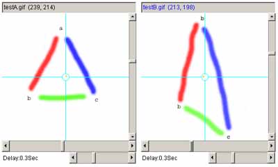
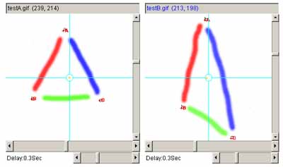
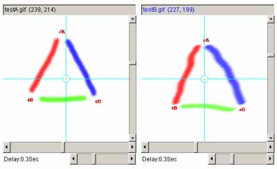
Figure 11. Example using the affine transform.
a) shows the original left and right images. b) shows
the left and right images with 3 pairs of landmarks after they are
added (large red A, B and C labels). c) shows the two images
after applying the affine transform to the right image and recentering
it.
6.6 Quantify menu
These commands are used to define and measure integrated density
(grayscale or calibrated OD if calibrated) for circle, boundary,
region-of-interest (ROI) measurements. Integrated density
measurements are made on the 8-bit (0:255 gray-value) data of
pixels. It is only valid on grayscale data since we do the
measurements on the least significant 8-bits (blue channel of the
24-bit RGB data). If you have color data, you can use the NTSC color
to gray-scale transform to convert it to gray scale first. If you
have calibrated grayscale to optical density (OD), you get the
measurement in terms of OD rather than grayscale. The calibration
wizard also lets you define the calibration in terms of other
unitsy.Creating lists of spots
Flicker was not designed to measure very large numbers of spots. That
said, it could be used that way but with a lot of manual work. We
provide some commands to make it easier to quantify (C-B) and
(C-M) or (ALT-click), annotate (C-I), edit
(C-E), and delete (C-K). You can also list and save the
measured spot lists for the two images. The measured spot lists
automatically get saved if you save the .flk startup state (File |
SaveAs state file). Opening Flicker using that startup state file
will restore the measured spot list.
-
region of interest operations
![]() - measure
intensity/density within the circlular mask
- measure
intensity/density within the circlular mask
![]() Use measurement counter) is
enabled. An alternative way to measure spots is to hold the
ALT-key when you press the mouse to select the spot. This
combines spot selection and measurement in one operation. Note
that you can toggle between trial- mode and spot-list measurement
mode using the (Quantify |
Use measurement counter) is
enabled. An alternative way to measure spots is to hold the
ALT-key when you press the mouse to select the spot. This
combines spot selection and measurement in one operation. Note
that you can toggle between trial- mode and spot-list measurement
mode using the (Quantify | ![]() List-of-spots else trial-spot measurement-mode (C-J)) checkbox
command.
List-of-spots else trial-spot measurement-mode (C-J)) checkbox
command.
------------------------------------
------------------------------------
![]() - measure
intensity/density within user-drawn boundary
- measure
intensity/density within user-drawn boundary
------------------------------------
![]() - Print
data-window
- Print
data-window
![]() 20x20 - window size
20x20 - window size
![]() Decimal - data format radix
Decimal - data format radix
------------------------------------
![]() - calibrate
optical density or other step wedge
- calibrate
optical density or other step wedge
![]() Use demo leukemia gels ND wedge
calibration preloads wedge - used to demonstrate the ND step
wedge calibration process. We have built in four sample ROI's and
the corresponding OD values corresponding to the step wedge scanned
with the four demo gels (Leukemia-AML, Leukemia-ALL, Leukemia-CLL,
Leukemia-HCL). Enable this option before invoking the
Optical density by step wedge command.
Use demo leukemia gels ND wedge
calibration preloads wedge - used to demonstrate the ND step
wedge calibration process. We have built in four sample ROI's and
the corresponding OD values corresponding to the step wedge scanned
with the four demo gels (Leukemia-AML, Leukemia-ALL, Leukemia-CLL,
Leukemia-HCL). Enable this option before invoking the
Optical density by step wedge command.
------------------------------------
------------------------------------
------------------------------------
![]()
------------------------------------
![]() List-of-spots else trial-spot
measurement-mode (C-J) to either measure spots or use a trial
measurement mode. In measurement mode, add spot label overlays
consisting of measurement locations (either "+" or circles or
neither) followed by measurement annotation (measurement # and/or
spot specific identifier (if edited), or neither). As specified by
the (View | Set view measurement options | ... checkbox
options. In measurement mode it will number the measurements 1, 2,
3, ... etc, whereas in trial-measurement mode it will show a
single "+M" instead. Note that in trial mode, it will redraw the
measurement circle as you change the size with the slider. Note
that if you are measuring several different ROI's with
(C-R), then it will assign sequential measurment numbers to
these ROI measurements.
List-of-spots else trial-spot
measurement-mode (C-J) to either measure spots or use a trial
measurement mode. In measurement mode, add spot label overlays
consisting of measurement locations (either "+" or circles or
neither) followed by measurement annotation (measurement # and/or
spot specific identifier (if edited), or neither). As specified by
the (View | Set view measurement options | ... checkbox
options. In measurement mode it will number the measurements 1, 2,
3, ... etc, whereas in trial-measurement mode it will show a
single "+M" instead. Note that in trial mode, it will redraw the
measurement circle as you change the size with the slider. Note
that if you are measuring several different ROI's with
(C-R), then it will assign sequential measurment numbers to
these ROI measurements.
6.6.1 Spot measurements
Figures 12a-12h show various permuations of the viewing spot
quantification using the various spot list overlay options.
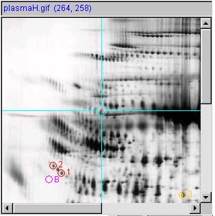
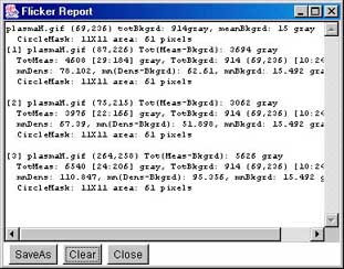
a.1)
a.2
b.1)
b.2)
c)
d)
e)
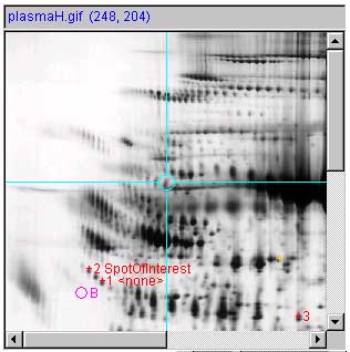
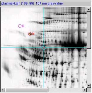
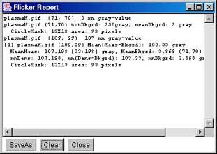
f)

g)
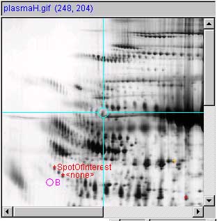
h)

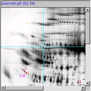
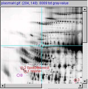
Figure 12. Examples of the measured spotlist.
This figures show various options in displaying the measured spots.
As a shorthand for this legend, VM: is the (View | Set view
measurements options | ...) submenu.![]() List-of-spots else
trial-spot measurement-mode (C-J)) should be turned off. The
VM:
List-of-spots else
trial-spot measurement-mode (C-J)) should be turned off. The
VM: ![]() View measurement circle
option should be enabled.
View measurement circle
option should be enabled.
Panels (b.1) and (b.2) show a measured spot list with
three spots, image and report respectively. Spots are shown with
circles and spot number annotation. Since the user had clicked on the
third spot, it is considered the "current" spot in the spot list and
is indicated in yellow. The rest are indicated in red. The
(Quantify | ![]() List-of-spots else
trial-spot measurement-mode (C-J)) should be turned on. The VM:
List-of-spots else
trial-spot measurement-mode (C-J)) should be turned on. The VM:
![]() Use 'circle' for measured spot
locations option should be turned on, VM:
Use 'circle' for measured spot
locations option should be turned on, VM: ![]() Use 'spot number, for spot annotations
option should be turned on.
Use 'spot number, for spot annotations
option should be turned on.
Panel (c) shows the measured spot list with a "+" instead of a
circle with spot numbers. Since the user had clicked on a different
part of the screen, there is no "current" spot in the spot list so all
spots are shown in red. The (Quantify | ![]() List-of-spots else trial-spot
measurement-mode (C-J)) should be turned on. The VM:
List-of-spots else trial-spot
measurement-mode (C-J)) should be turned on. The VM: ![]() Use '+ for measured spot locations
option should be turned on, VM:
Use '+ for measured spot locations
option should be turned on, VM: ![]() Use
'spot number, for spot annotations option should be turned on.
Use
'spot number, for spot annotations option should be turned on.
Panel (d) show a measured spot list with three spot
measurements image and report. Spots are shown with circles, spot
numbers and spot annotation. The (Quantify | ![]() List-of-spots else trial-spot
measurement-mode (C-J)) should be turned on. The VM:
List-of-spots else trial-spot
measurement-mode (C-J)) should be turned on. The VM: ![]() Use 'circle' for measured spot
locations option should be turned on, VM:
Use 'circle' for measured spot
locations option should be turned on, VM: ![]() Use 'spot number, for spot annotations
option should be turned on, and VM:
Use 'spot number, for spot annotations
option should be turned on, and VM: ![]() Use 'spot identifier, for spot
annotations option should be turned on. The user had edited the
spot identifiers by (1) clicking on a spot, (2) doing the (Quantify
| Measure by circle | Edit selected spot from spot list (C-E))
command, and 3) typing a spot "identifier" for that spot and pressing
"Done". Spots where the 'id was not edited are indicated by
"<none>". For this example, we set 'id' to "SpotOfInterest" for
spot #1 and a space for spot #3. Spaces make the identifier disappear.
Use 'spot identifier, for spot
annotations option should be turned on. The user had edited the
spot identifiers by (1) clicking on a spot, (2) doing the (Quantify
| Measure by circle | Edit selected spot from spot list (C-E))
command, and 3) typing a spot "identifier" for that spot and pressing
"Done". Spots where the 'id was not edited are indicated by
"<none>". For this example, we set 'id' to "SpotOfInterest" for
spot #1 and a space for spot #3. Spaces make the identifier disappear.
Panel (e) show a measured spot list with three spot
measurements image and report. Spots are shown with pluses, spot
numbers and spot annotation. The (Quantify | ![]() List-of-spots else trial-spot
measurement-mode (C-J)) should be turned on. The VM:
List-of-spots else trial-spot
measurement-mode (C-J)) should be turned on. The VM: ![]() Use '+' for measured spot locations
option should be turned on, VM:
Use '+' for measured spot locations
option should be turned on, VM: ![]() Use
'spot number, for spot annotations option should be turned on, and
VM:
Use
'spot number, for spot annotations option should be turned on, and
VM: ![]() Use 'spot identifier, for spot
annotations option should be turned on.
Use 'spot identifier, for spot
annotations option should be turned on.
Panel (f) show a measured spot list with three spot
measurements image and report. Spots are shown with circles and spot
annotation. The (Quantify | ![]() List-of-spots else trial-spot
measurement-mode (C-J)) should be turned on. The VM:
List-of-spots else trial-spot
measurement-mode (C-J)) should be turned on. The VM: ![]() Use 'circle' for measured spot
locations option should be turned on, and VM:
Use 'circle' for measured spot
locations option should be turned on, and VM: ![]() Use 'spot identifier, for spot
annotations option should be turned on.
Use 'spot identifier, for spot
annotations option should be turned on.
Panel (g) show a measured spot list with three spot
measurements image and report. Spots are shown with pluses and spot
annotation. The (Quantify | ![]() List-of-spots else trial-spot
measurement-mode (C-J)) should be turned on. The VM:
List-of-spots else trial-spot
measurement-mode (C-J)) should be turned on. The VM: ![]() Use '+' for measured spot locations
option should be turned on, and VM:
Use '+' for measured spot locations
option should be turned on, and VM: ![]() Use 'spot identifier, for spot
annotations option should be turned on.
Use 'spot identifier, for spot
annotations option should be turned on.
Panel (h) show a measured spot list with three spot
measurements image and report. Spots are shown with just spot
annotation. The (Quantify | ![]() List-of-spots else trial-spot
measurement-mode (C-J)) checkbox option should be turned on. The
VM:
List-of-spots else trial-spot
measurement-mode (C-J)) checkbox option should be turned on. The
VM: ![]() Use 'spot identifier, for spot
annotations option should be turned on.
Use 'spot identifier, for spot
annotations option should be turned on.
6.6.2 Region of Interest histogram display
You can compute a histogram of the current region of interest in the
selected image. Figure 13 shows an example of a histogram of the
Region Of Interest (ROI).
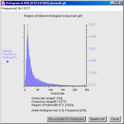
Figure 13. Example of a grayscale histogram of a region in the
image. This popup window shows the grayscale
histogram under the computing window region of interest (ROI). If no
ROI was defined (the case shown here), it computes the histogram over
the entire image. It is invoked by (Quantify | Region Of Interest
(ROI) | Show RPI grayscale histogram (C-H)). Clicking on a value
of the histogram will show the frequency of the specified gray value
at the top of the display.
6.6.3 The ND step wedge grayscale calibration
[ALPHA-level code]
It is useful and sometimes essential to
calibrate an image using known standard density values. If the gel
stain is stoichiometric within limits, density corresponds to protein
concentration. Then within the contraints of linearity of the
staining, range and saturation of the scanner, it is possible to get
more accurate spot density measurements. One way to do do this is to
scan the gel (or image) with a neutral density step wedge (Suppliers:
such as Stauffer Graphic Arts or similar) with known optical density
(OD) values for each step. Note that if you have step wedges
calibrated in other units (e.g., counts-per-minute or CPM, then you
can specify that to the calibration wizard). If the gray values are
mapped to the corresponding optical density values, the wizard
interpolates the intervening values constructing a translation table
to map gray scale (in the range of [0:255] used in Flicker) to the
coresponding OD or other calibration values. Then when measurements
are made using the Quantify menu commands (circle mask or ROI), the
data is first mapped to the calibrated units rather than grayscale.
The sum of the pixel gray values is computed using this map so the
measurement is the sum of the optical densities or integrated
density/spot measurement area. This gives a better estimate of the
protein concentration. Procedure: for calibrating the ND step wedge
4.1 It tries to find the peaks and copies the peaks into the
Calibration Peak Table Gray-peak fields.
4.2 It then generates a piecewise-linear extrapolation of the
peak-table data to generate the translation map.
4.3 It then redraws the histogram plot with
a) overlay calibration curve which is the gray to OD map,
b) updates the peaks table of (OD values,
peak gray values) and draws this data into the plot.
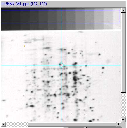
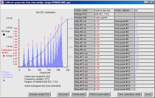
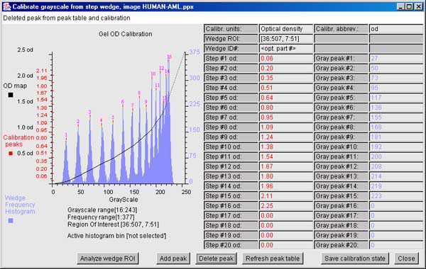
Figure 14. Example of calibrating grayscale using the step wedge
calibration wizard. This shows an example of
calibrating the gray scale using a ND step wedge that was scanned with
the image. The OD values corresponding to the steps are known and are
entered into the peak table. a) The ROI region over the ND step
wedge was defined. In this example using one of the demo leukemia gels
(AML), we used the preload option (Quantify | Calibration | Use
demo leukemia gels ND wedge calibration preloads) command. Then,
startup the wizard by using the (Quantify | Calibration | Optical
density by step wedge) command. If you did not do this, then you
must define the ROI for the wedge region yourself and then press the
Analyze wedge ROI button. b) Shows the calibration
wizard window with the histogram on the left, the peak table on the
right and control buttons on the bottom. This is before editing the
histogram. If you were defining the calibration values from scratch,
enter them in the peak table and define the calibration units and
units abbreviation. Then press the Update peak table button.
c) Because there are some bad peaks (#7, grayscale of 143) and
some that were missed (grayscale peaks at 214 and 220), we need to
edit the peak table. Click on each peak in the histogram you want to
delete and then press the Delete peak button. To add peaks,
click on each peak in the histogram you want to add and then press the
Add peak button. When you are satisfied with the calibration,
press the Save calibration file to save the calibration in the
{installation directory}/cal/{imageName}.cal file and then
press Close to exit the wizard. A good calibration should be a
smooth continuous function with no kinks. If you forgot to save the
calibration when you leave the wizard, it will ask you if you want to
save it. If you don't, it will revert to the previous calibration if
any.
6.6.4 The Spot list grayscale calibration
[ALPHA-level code]
There is an alternative calibration method. You can calibrate
grayscale if have a set of calibrated spots or regions in the image
instead of a calibration step-wedge. You do not use the ROI, but
instead will specify a set of spot measurements of increasing darker
regions that correspond to your calibration values (such as OD, CPM,
etc). (Quantify | Calibration | Optical density by spot list)
command. This will popup the calibration wizard window.
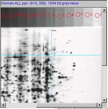
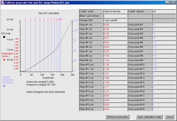
Figure 15. Example of calibrating grayscale using the spot list
calibration wizard. This shows an example of
calibrating the gray scale using a set of known calibrated regions or
spots that were scanned with the image. The OD or other calibration
values corresponding to the spots are known and are entered into the
peak table. a) We selected a set of spots over the ND step
wedge but any set of known regions could be used. In this example
using one of the demo leukemia gels (AML), we used the preload option
(Quantify | Calibration | Use demo leukemia gels ND wedge
calibration preloads) command. Then, startup the wizard by using
the (Quantify | Calibration | Optical density by spot list)
command. If you did not do this, then you must define the OD list of
calibration values yourself and then press the Update peak
table button. b) Shows the calibration wizard window with
the histogram on the left, the peak table on the right and control
buttons on the bottom. If you are defining the calibration values from
scratch, enter the OD (or other calibration values) into the peak
table and define the calibration units and units abbreviation. Then
press the Update peak table button. You may edit the peak tale
(just as you can for the ND wedge calibration). When you are
satisfied with the calibration, press the Save calibration file
to save the calibration in the {installation
directory}/cal/{imageName}.cal file and then press Close
to exit the wizard. A good calibration should be a smooth continuous
function with no kinks. If you forgot to save the calibration when you
leave the wizard, it will ask you if you want to save it. If you
don't, it will revert to the previous calibration if any.
6.6.5 Example of measuring multiple spots using the circular mask
This gives an example of how do you can measure spot intensity under
the circular mask. First, the background corrected measurement
estimate is computed under the circular mask (C-M). This
background estimate is then used for multiple measurements until you
change this background estimate. The current background intensity
measurement is associated with all spots measured since it was defined
or redefined and is saved in the spot list. You number the spots by
enabling the (View menu | Set view measurement options | ![]() View measurement circle) option. The
numbered image is shown in Figure 16a.
View measurement circle) option. The
numbered image is shown in Figure 16a.
![]() List-of-spots else trial-spot
measurement-mode (C-J)) menu checkbox.
List-of-spots else trial-spot
measurement-mode (C-J)) menu checkbox.
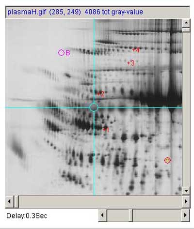
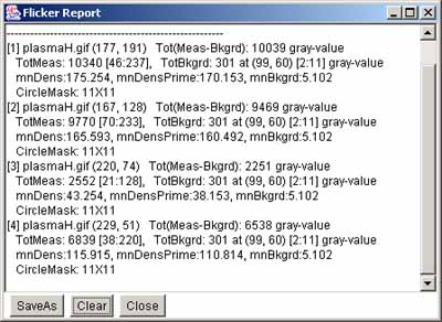
Figure 16. Example of measuring multiple spots.
a) shows the left image window with 4 spots measured. The
background spot has a magenta circle and "+B". The 4 spots are
numbered "+1", "+2", to "+4". The current cursor position is shown
with the red circle with an orange "+" inside of it and the total gray
value shown in the image title is the data under the circular mask at
this position. b) shows the popup report window with the 4
spot measurements. We "Clear"ed the report to before posting the data
to have it contain just the spot data.
6.6.6 Examples of annotating spot 'ID's in the spot lists
Flicker allows you to annotate spots in the spot list and to then
generate paired-spot tables (tab-delimited) that you can export (to
Excel etc.). Figure 17 shows 3 spots that were
putatively identified by flickering the right gel against the
Swiss-2DPAGE database image and then clicking on each of the
corresponding spots to bring up the putative identifications (see Figure 2). Once the paired spot identifications are
assigned,
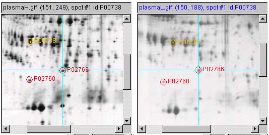

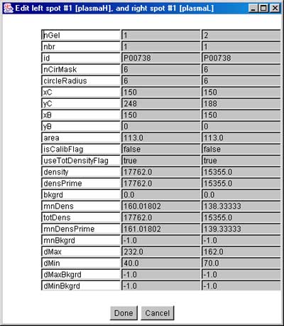
Figure 17. Example of assigning spot annotation 'id's. a) shows the labeled spot annotations for three spots
previously putatively identified (not shown here) using flickering
against the SWISS-2DPAGE clickable database (see Figure 2). The spots were added to the spot lists in
each of the two gels using the (Quantify | Measure by circle |
Capture measurement (C-M)) command on each spot. Then, b)
shows the prompt for assigning the paired-spot identifier that is
popped up by first selecting the corresponding measured spots in each
gel (shown in yellow) and then using the (Quantify | Measure by
circle | Edit selected spot(s) 'id' field from spot list(s) (C-I))
command. An alternate editing method, c) shows the prompt for
editing all fields of the paired-spots that is popped up by first
selecting the corresponding measured spots in each gel (shown in
yellow) and then using the (Quantify | Measure by circle | Edit
selected spot(s) from spot list(s) (C-E)) command.
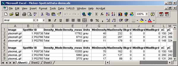


Figure 18. Example of paired spot lists exported to Excel.
a.1-a.2) shows data exported to Excel from the
above example (Figure 17). The annotated (ids')
spot lists were generated by clicking (for each gel) on the image then
using the (Quantify | Measure by circle | List spots in the spot
list (tab-delimited)) command to generate a tab-delimited spot
this. This was then cut and pasted into Excel and then reorganized to
better show the data for this Web page. Then, b.1-b.2) shows
the paired spot table generated using the (Quantify | Measure by
circle | List 'id'-paired annotated mean norm. spots in both spot
lists (tab-delimited)) command. The table was then cut and pasted
into Excel and then reorganized to better show the data for this Web
page.
6.6.7 Examples of typical print-data windows
A spot was first selected by clicking on it. The print window size was
set to 20x20 and the data radix to Decimal for grayscale
values. Then the following output was generated in the popup Report
window using the (Quantify menu | Print data-window | Show
data-window of selected pixel (C-V)) command. Normally, first set
the print-window size and data radix then use the (C-V)
short-cut key after you have selected the spot you want to view. The
following shows typical output for an uncalibrated image where you can
see tow spots in the lower left quadrant:
Windmp [183:203, 168:188] Center (193,178) 20X20 size,
sampled: 1 pixels, data-radix: Decimal
Image: Images\plasmaH.gif
    X 183 184 185 186 187 188 189 190 191 192 193 194 195 196 197 198 199 200 201 202 203
  Y   --- --- --- --- --- --- --- --- --- --- --- --- --- --- --- --- --- --- --- --- ---
 168   71  61  57  55  54  54  56  57  56  50  46  42  42  43  45  42  43  48  53  67  80
 169   71  53  50  48  45  48  50  55  60  56  46  42  40  43  42  40  37  41  47  54  65
 170   88  49  44  42  40  42  45  53  56  61  50  41  40  39  39  37  34  37  38  45  54
 171   97  49  41  39  39  40  43  53  60  61  54  43  39  38  37  36  34  36  37  43  50
 172  106  47  39  37  36  37  39  53  72  78  72  50  43  38  37  35  33  34  35  39  44
 173   84  41  38  37  34  33  35  50  82  94  84  58  48  41  40  37  34  35  35  39  44
 174   66  39  38  37  35  33  35  50  84  96  84  59  48  41  40  39  35  37  37  39  44
 175   47  41  43  40  36  34  34  49  78  84  71  56  50  43  44  43  38  37  37  47  46
 176   50  46  46  46  39  34  35  56  91  95  77  61  58  54  57  54  47  43  41  43  47
 177   53  49  51  50  42  37  38  69 117 122  98  74  66  62  65  62  51  47  44  45  50
 178   58  59  65  65  53  43  46 106 171 174 139  94  78  71  67  65  57  54  50  48  54
 179   63  77  97  97  82  59  55 104 163 164 120  76  64  58  62  62  61  58  55  52  56
 180   67  90 122 124 106  72  60  86 132 132  95  64  59  55  64  62  61  59  57  53  57
 181   76 140 189 193 174 128  94  59  70  68  60  55  55  54  59  63  60  60  58  55  58
 182   82 167 214 215 195 137  97  50  47  49  52  53  53  53  53  56  55  57  59  57  61
 183   73 142 194 194 160  97  67  42  44  46  51  52  52  50  53  52  54  57  60  62  63
 184   51  62  81  80  60  46  39  38  44  46  51  52  52  51  54  54  66  69  78  80  77
 185   48  50  52  52  46  40  39  40  45  48  51  52  51  53  56  57  56  65  70  72  72
 186   49  49  50  50  46  41  40  40  42  46  49  51  51  53  55  56  53  62  60  61  61
 187   51  55  63  62  56  46  43  40  40  41  45  51  53  57  58  55  50  48  52  49  50
 188   70  90  97  90  71  57  52  47  41  40  46  56  61  66  64  60  51  46  48  47  50
Example of a print-data window from an OD calibrated gel
If you have a calibrated image (see (Quantify menu | Calibrate |
...), then you can view the calibrated pixels in an OD radix. The
following AML demo leukemia gel was calibrated in optical density.
The spot was first selected by clicking on it. The print window size
was set to 20x20 and the data radix to Optical-density for od
values. Then the following output was generated in the popup Report
window using the (Quantify menu | Print data-window | Show
data-window of selected pixel (C-V)) command. Normally, first set
the print-window size and data radix then use the (C-V)
short-cut key after you have selected the spot you want to view. The
following shows typical output for an uncalibrated image:
Windmp [183:197, 322:336] Center (190,329) 15X15 size,
sampled: 1 pixels, data-radix: Optical-density
Image: Images\HUMAN-AML.ppx
    X   183   184   185   186   187   188   189   190   191   192   193   194   195   196   197
  Y   ----- ----- ----- ----- ----- ----- ----- ----- ----- ----- ----- ----- ----- ----- -----
 322  0.022 0.022 0.027 0.033 0.038 0.056 0.066 0.072 0.084 0.056 0.049 0.047 0.033 0.040 0.047
 323  0.018 0.022 0.020 0.042 0.058 0.058 0.097 0.139 0.090 0.066 0.053 0.029 0.027 0.029 0.036
 324  0.020 0.013 0.024 0.040 0.049 0.051 0.127 0.133 0.072 0.060 0.058 0.038 0.036 0.042 0.033
 325  0.018 0.027 0.038 0.038 0.078 0.127 0.151 0.157 0.145 0.072 0.049 0.040 0.042 0.033 0.038
 326  0.024 0.022 0.033 0.066 0.139 0.188 0.291 0.304 0.265 0.115 0.056 0.040 0.038 0.031 0.033
 327  0.018 0.029 0.047 0.109 0.265 0.401 0.534 0.495 0.337 0.194 0.078 0.031 0.029 0.036 0.029
 328  0.038 0.029 0.058 0.182 0.394 0.665 0.766 0.648 0.466 0.252 0.097 0.058 0.033 0.022 0.022
 329  0.027 0.031 0.066 0.239 0.495 0.724 0.816 0.674 0.522 0.272 0.121 0.051 0.027 0.024 0.024
 330  0.036 0.044 0.127 0.220 0.394 0.557 0.622 0.557 0.372 0.246 0.139 0.040 0.033 0.038 0.027
 331  0.027 0.036 0.060 0.145 0.291 0.394 0.394 0.357 0.291 0.176 0.066 0.038 0.031 0.029 0.031
 332  0.024 0.033 0.044 0.090 0.133 0.233 0.285 0.246 0.207 0.151 0.090 0.058 0.056 0.042 0.049
 333  0.027 0.018 0.042 0.060 0.115 0.170 0.239 0.239 0.246 0.182 0.157 0.188 0.145 0.145 0.182
 334  0.018 0.031 0.044 0.051 0.097 0.157 0.252 0.304 0.272 0.291 0.246 0.233 0.291 0.317 0.365
 335  0.033 0.031 0.042 0.058 0.151 0.176 0.259 0.311 0.343 0.343 0.324 0.298 0.291 0.350 0.430
 336  0.018 0.036 0.056 0.090 0.139 0.252 0.291 0.304 0.357 0.298 0.265 0.246 0.272 0.265 0.317
6.7 Help menu
These commands are used to invoke popup Web browser documentation on
Flicker. The documentation is kept on the Internet at
http://open2dprot.sourceforge.net/Flicker. Normally, these help
commands should pop up a Web browser that directly points to the Web
page on the http://open2dprot.sourceforge.net/Flicker site. If your
browser is not configured correctly, it may not be able to be launched
directly from the Flicker program. Instead, just go to the Web site
with your Web browser and look up the information there.
![]() -
this reference manual
-
this reference manual
![]()
![]()
7. Demonstrations
The Flicker program integrates these various procedures to help you
try to make putative spot identifications. See the Quick start examples on the home
page for a short list of some of these methods.8. Flicker References
Contact us
Flicker is a contributed program available at
open2dprot.sourceforge.net/Flicker
Powered by
Revised: 05/12/2007